
A modular, cross-platform framework for automated DCE-MRI and diffusion MRI research.

Project description
p-Brain
A Modular Open-Source Framework for
Automated Quantitative DCE-MRI of Cerebral Perfusion,
Microvasculature, and Blood-Brain Barrier Permeability




p-Brain (the "p" stands for perfusion and permeability) is a
cross-platform Python command-line tool for quantitative DCE-MRI. Install it with
pip on Linux, macOS, or Windows (Python 3.10 to 3.12), point pbrain run at a
subject's scans, and it produces the full derivatives tree. No notebook, GUI, or
server is required. The command-line tool is the product. An optional macOS
desktop application is one front-end built on top of it (see
below).
p-Brain takes raw dynamic-contrast-enhanced, and optionally diffusion, MRI through the complete analysis: T1/M0 mapping, arterial-input-function extraction, signal-to-concentration conversion, tissue parcellation, and pharmacokinetic and diffusion modelling. It produces standardised voxel-, tissue-, and parcel-level results automatically.
p-Brain serves two purposes. As shipped, it is a validated, ready-to-run
pipeline that you can point at real scanner data to obtain quantitative maps
(Ki, CBF, MTT, CTH, FA, and others). It is also a framework you extend. Each
step is a self-contained plug-in, so adding your own kinetic model, a different
AIF, a segmentation backend, or a whole stage means writing a single file with
no changes to the core. Drop a model into pbrain/models/, call it with
--models yourmodel, and it runs on every subject, is aggregated to every
anatomical level, is written as NIfTI, CSV, and JSON, and is given diagnostics
automatically.
The goal is to let groups reuse a common, tested pipeline instead of re-implementing the same steps, so that outputs stay directly comparable across studies.
If you use p-Brain in your research, please cite our paper (Tireli et al., see Citation).
Author: Edis Devin Tireli, M.Sc., Ph.D. student Affiliations: Functional Imaging Unit, Copenhagen University Hospital, Rigshospitalet. Department of Neuroscience and Department of Clinical Medicine, University of Copenhagen.
Contents
- Why a framework
- Install
- Try it: the example subject
- How to run
- Add your own model
- Config files
- Models
- Diffusion and connectomics
- Outputs
- Representative output
- Demo
- Repository structure
- Documentation
- Citation
Why a framework
DCE-MRI analysis is a chain of stages: fit T1, find the artery, convert signal to contrast concentration, segment tissue, fit a kinetic model, and summarise. In most labs each of these is bespoke code, which makes results hard to compare and turns a new model into a rewrite of the whole pipeline.
p-Brain makes each stage a plug-in, a single file that declares what it needs and what it produces and is discovered automatically at runtime. The orchestrator wires the stages together from those declarations, so that:
- adding a method changes one file and never the core,
- every model is run, aggregated, and reported the same way, which gives standardised, directly comparable outputs across groups,
- you can swap any step, such as a different AIF, your lab's segmentation tool, or a new deconvolution, by name on the command line.
There are 12 such plug-points. The full contract and copy-paste templates are in
docs/ADDING_PLUGINS.md,
and the design rationale is in
docs/ARCHITECTURE.md.
Read those two when you want to extend the framework. The rest of this README
gets you running first.
Install
p-Brain is a standard pip-installable Python package. It runs on Linux,
macOS, and Windows with Python 3.10 to 3.12.
pip install p-brain
pbrain --help
This installs the pbrain command, also available as python -m pbrain,
together with the light core dependencies (numpy, scipy, matplotlib, nibabel).
Everything heavier is an opt-in extra, installed only when you select a plug-in
that needs it:
pip install "p-brain[cnn]"        # TensorFlow, for the CNN arterial-input-function (default AIF)
pip install "p-brain[diffusion]"  # dipy, for the diffusion track (DTI, DKI, CSD, and others)
pip install "p-brain[dicom]"      # pydicom, for DICOM input (see DICOM input below)
pip install "p-brain[all]"        # all extras at once
The default AIF (cnn_sss_shifted) needs the CNN extra and its trained .keras
weights (about 1.2 GB), which are archived on Zenodo. Download them once. They
cache under ~/.p-brain/AI, and every later run finds them automatically:
pbrain setup            # interactive: installs extras and offers to fetch weights and data
pbrain fetch-weights    # the CNN weights only        (Zenodo 10.5281/zenodo.15697443)
pbrain fetch-data       # the example subject sub-01  (Zenodo 10.5281/zenodo.20826857)
To run without any weights, supply a file-based or model-free AIF. Use
--aif curve_file for a saved curve as in the example, from_file or manual
for your own ROIs, or deterministic for a DCE-only synthetic AIF. You can also
run python -m pbrain.demo, which needs no weights or data at all.
From source, for development:
git clone https://github.com/edtireli/p-brain.git
cd p-brain
pip install -e ".[dev]"
pytest -q
Check your environment. python -m pbrain check-deps verifies the
third-party Python dependencies and offers to install any that are missing.
python -m pbrain setup additionally inspects external tooling (dcm2niix,
optionally FreeSurfer for segmentation, and GPU support) and walks you through it.
DICOM input
p-Brain reads NIfTI (.nii or .nii.gz) and Philips PAR/REC natively.
DICOM is supported through
dcm2niix, the standard, well-validated
DICOM-to-NIfTI converter. Point --dce, --ir, or --dwi at a DICOM file or a
folder of DICOMs, and p-Brain calls dcm2niix under the hood and picks up the
reconstructed NIfTI, and, for diffusion, the .bval and .bvec gradient tables
it writes.
Install dcm2niix from its own channel. It is a compiled binary, not a pip
package:
conda install -c conda-forge dcm2niix     # any OS (recommended)
brew install dcm2niix                      # macOS
sudo apt install dcm2niix                  # Debian / Ubuntu
# Windows: download the release .zip from the dcm2niix GitHub page and add it to PATH
pip install "p-brain[dicom]" adds pydicom for header inspection. dcm2niix
must be on your PATH for the actual conversion. Run
python -m pbrain check-deps to confirm it is found.
Optional macOS app
A native macOS desktop application wraps this command-line tool in a point-and-click interface for users who prefer not to use a terminal. It is entirely optional. The Python command-line tool described here is the product and the canonical interface, and the application simply drives it.
Try it: the example subject
This is the quickest way to confirm p-Brain works end-to-end, on Linux, macOS, or Windows, with no CNN weights and no FreeSurfer or SynthSeg. The example ships its own AIF curve and parcellation, so nothing extra is downloaded.
pip install p-brain
pbrain fetch-data          # downloads sub-01 (about 99 MB), then prints the exact run command
pbrain fetch-data locates the data and prints a ready-to-run, weights-free
command with the correct paths for your machine. Copy, paste, and run it. It has
the form:
python -m pbrain run \
  --subject-dir <data>/sub-01 \
  --dce  <data>/sub-01/sub-01_dce.nii.gz  --ir <data>/sub-01/sub-01_ir.nii.gz \
  --aif  curve_file      --opt aif.curve_file.curve_path=<data>/sub-01/sub-01_aif.npy \
  --tissue-roi preloaded --opt tissue_roi.preloaded.parcellation_path=<data>/sub-01/sub-01_parcellation.nii.gz \
  --models patlak,tikhonov --aggregations region,parcel,voxelwise
Results are written under sub-01/derivatives/. Compare
07_kinetic/patlak/region/ki.csv (BBB Ki and vb) and
07_kinetic/tikhonov/region/cbf.json (CBF and MTT) against the bundled
expected_outputs/. The values should agree to within about 2 percent.
Windows. The command is pure Python and runs the same way in PowerShell or
cmd. Put it on one line, or replace each trailing backslash with a backtick. You do not need dcm2niix, FreeSurfer, or the CNN weights to run the example.
No download at all. python -m pbrain.demo synthesises a small phantom and
runs the entire pipeline in seconds, a self-contained check that your install
works on any operating system.
How to run
A run takes one subject's raw data and produces its full derivatives tree. There are three choices to make.
- Point at your data.
--dceis the 4-D DCE series (NIfTI, PAR/REC, or DICOM, converted automatically).--iris the inversion-recovery series used to fit T1 and M0.--dwiis an optional diffusion scan. Each of--dce,--t1, and--iraccepts a full path, a filename, a protocol-name substring, orauto, so you can write--dce hperf --t1 auto --ir autoonce and reuse it across subjects whose scan numbers differ. Raw PAR/REC files are matched by their PhilipsProtocol name, and--ir autoassembles theTI_*series. - Choose your methods.
--models patlak,tikhonovselects the kinetic models.--aif,--tissue-roi, and--t1m0select how each upstream step is done. Sensible defaults mean you can omit most of them. - Choose your output levels.
--aggregations voxelwise,region,parcelcontrols whether you get whole-brain maps, tissue-class summaries, and per-parcel tables.
The flags
| flag | meaning | default |
|---|---|---|
--subject-dir |
where the derivatives tree is written | required |
--dce |
4-D DCE series (NIfTI, PAR/REC, or DICOM) | required |
--ir |
inversion-recovery series for the T1/M0 fit | none |
--dwi |
diffusion series, for the diffusion track | none |
--t1m0 |
how T1 and M0 are obtained (inversion_recovery, vfa_spgr, and others) |
inversion_recovery |
--aif |
arterial-input-function method | cnn_sss_shifted |
--tissue-roi |
parcellation source (synthseg, fastsurfer, command, preloaded, voxelwise) |
voxelwise |
--models |
comma-separated list of kinetic models to run | patlak,tikhonov |
--diffusion |
comma-separated list of diffusion models, or default or all |
auto when --dwi is given |
--aggregations |
output levels: voxelwise,region,parcel,slice_wise |
voxelwise,parcel,region |
--device |
cpu, mps, cuda, or auto |
cpu |
--config |
read all of the above from a .toml or .yaml file |
none |
Runs are resumable. A finished stage is skipped on re-run, and --force
recomputes it. Every output carries provenance, namely the pbrain version and
the exact options that produced it. Use --quiet, --verbose, or --log-file
to control logging.
Quick start
# Minimal: DCE and IR, the default models, all output levels
python -m pbrain run \
    --subject-dir /data/sub-01 \
    --dce dce.nii.gz --ir ir.nii.gz \
    --models patlak,tikhonov \
    --aggregations voxelwise,parcel,region

# With diffusion (FA, MD, and tractography) in the same command
python -m pbrain run \
    --subject-dir /data/sub-01 \
    --dce dce.nii.gz --ir ir.nii.gz --dwi dwi.nii.gz \
    --models patlak,tikhonov --diffusion default
See what is available, including every plug-in with its inputs, outputs, and diagnostics:
python -m pbrain list             # all plug-points at a glance
python -m pbrain list models      # one plug-point in detail
Run a whole cohort in parallel, resumable and error-isolated:
# One flag on raw scanner data: point --cohort at a folder of subjects.
# Each sub-directory is a subject of raw Philips PAR/REC. Inputs are
# auto-discovered by protocol name (DCE from hperf*, the TI_* saturation-recovery
# series assembled into an IR, and a 3-D T1 anatomical for SynthSeg). The full
# pipeline then runs with all kinetic models at tissue (region) and parcel level.
# No config is needed. Add --force for a fresh re-run. Pass several roots to run
# patients, controls, and follow-ups in one go.
python -m pbrain run-cohort --cohort /data/patients /data/controls --workers 4 --force

# Pick models or levels, or skip known-bad subjects:
python -m pbrain run-cohort --cohort /data/patients --workers 4 \
    --models tikhonov,inverse_gaussian --aggregations region,parcel \
    --exclude 20221003x1            # add --voxelwise to also fit per-voxel (slower)

# Config mode for pre-converted NIfTI cohorts: inputs come from a shared config.
python -m pbrain run-cohort --config study.toml --data-dir /data --workers 8
python -m pbrain run-cohort --config study.toml --subjects-glob '/data/sub-*' --workers 8
--cohort is the one-flag path for a whole study. It resolves each subject's
DCE, IR, and T1 itself, because scan numbers vary between subjects and cannot be
templated by name, and it fits every model at the parcel level by default. That
is average-then-fit, which is the resolution these models support and is
tractable across hundreds of subjects. Use --config mode when inputs are
already NIfTI and named consistently.
Override any option with --opt <plug-point>.<plugin>.<key>=<value>, for
example --opt models.tikhonov.lambda_selection=evidence. Every option is
documented under Models.
Add your own
Step-by-step guide:
docs/ADDING_PLUGINS.mdhas templates for models, AIF methods, segmentation backends, diffusion models, and whole pipeline stages. Start there.
A new kinetic model is one file with no core changes. You write the mathematics, and the framework runs it on every voxel and curve, aggregates the result to tissue classes and parcels, writes NIfTI, CSV, and JSON, and renders fit diagnostics.
pbrain/models/two_cxm.py:
from dataclasses import dataclass
from typing import Any, ClassVar
import numpy as np
from .base import CurveInputs, ModelResult

@dataclass(frozen=True, slots=True)
class TwoCXM:
    key:         ClassVar[str] = "two_cxm"            # the name you call it by
    name:        ClassVar[str] = "Two-compartment exchange model"
    description: ClassVar[str] = "Fp, PS, vp, ve via 2CXM least-squares."
    outputs:     ClassVar[tuple] = ("fp", "ps", "vp", "ve")
    units:       ClassVar[dict]  = {"fp": "mL/100g/min", "ps": "mL/100g/min",
                                    "vp": "fraction", "ve": "fraction"}

    def fit(self, inputs: CurveInputs, **opts: Any) -> ModelResult:
        ...                                            # your maths -> fp, ps, vp, ve
        return ModelResult(maps={"fp": fp, "ps": ps, "vp": vp, "ve": ve},
                           units=dict(self.units))

PLUGIN = TwoCXM()
That is the entire integration. Now:
python -m pbrain run --models two_cxm,patlak ...
runs your model alongside Patlak, produces fp, ps, vp, and ve maps,
aggregates each to region and parcel level, and draws per-tissue fit plots,
all automatically.
The step-by-step guide for this and the other 11 plug-points (AIF methods,
segmentation backends, diffusion models, and whole stages) is
docs/ADDING_PLUGINS.md.
Start there.
Config files
For reproducibility, put the whole run in a versioned file and call
pbrain run --config study.toml. Command-line flags still override it.
subject_dir = "/data/sub-01"

[inputs]
dce = "dce.nii.gz"
ir  = "ir.nii.gz"
dwi = "dwi.nii.gz"

[pipeline]
t1m0         = "inversion_recovery"
aif          = "cnn_sss_shifted"
tissue_roi   = "synthseg"
models       = ["patlak", "tikhonov"]
diffusion    = "default"
aggregations = ["region", "parcel"]

[acquisition]
flip_angle_deg = 30.0
tr_s           = 0.01118

[options]                                  # same keys as --opt
"models.tikhonov.lambda_selection" = "evidence"
TOML works out of the box. YAML needs pip install pyyaml.
Models
Set any option with --opt models.<key>.<opt>=<value>, or in a config file.
Defaults are what you get without setting anything.
patlak produces blood-brain-barrier influx Ki and blood volume vp
from the Patlak graphical analysis.
| option | default | what it does |
|---|---|---|
regression |
huber |
slope fit. huber is robust to leverage points, ols is ordinary least squares. |
tail_mode |
smart |
which late points enter the fit. smart detects the linear tail from curvature, legacy uses a fixed upper two-thirds window. |
aif_min_fraction |
0.05 |
drop AIF samples below this fraction of the peak, which avoids a near-zero AIF inflating Ki. |
tikhonov produces CBF, MTT, and CTH by regularised deconvolution of the
residue function.
| option | default | what it does |
|---|---|---|
lambda_selection |
gcv |
regularisation strength. gcv uses cross-validation, lcurve uses the L-curve, and evidence uses the marginal likelihood, which is the most robust on smooth curves. |
lambda_spacing |
log |
lambda grid spacing (log or linear). |
n_lambdas |
121 |
number of lambda values searched. |
mtt_cth_method |
residue_integral |
MTT and CTH from the residue integral or the central-volume theorem. |
extended_tofts produces Ktrans, ve, vp, and kep by constrained
Levenberg-Marquardt fitting, with no tuning needed for the default fit.
This list is meant to be extended. See Add your own.
Diffusion
Give a diffusion scan with --dwi (NIfTI, PAR/REC, or DICOM, converted
automatically with gradients extracted) and the diffusion track runs in native
DWI space and resamples to your parcellation. Select models with --diffusion
(dti, a comma-separated list, default for shell-aware selection, or all),
and set options with --opt diffusion.<key>.<opt>=<value>.
Which model to use
dtiproduces FA, MD, AD, and RD and colour-FA. It works with any DWI that has a b0 and one shell, and is the place to start for FA and MD.dkiadds mean, axial, and radial kurtosis and KFA. It needs at least 2 shells.dki_microproduces WMTI microstructure (axonal water fraction, tortuosity) and μFA. Multi-shell.fwdtiperforms free-water elimination, giving tissue FA and MD with CSF and oedema removed, plus the free-water fraction. Multi-shell.csdperforms constrained spherical deconvolution, giving fibre orientations for tractography and GFA. Multi-shell is preferred.rsiproduces restriction-spectrum fractions (restricted, hindered, free). It needs a high-b shell.noddiproduces neurite density and orientation dispersion. It needs AMICO and a high-b shell.
Connectomics: tractography and connectome
With a fibre-orientation model, csd by default or the dti tensor, the
diffusion track can run tractography and build a structural connectome
between parcels:
python -m pbrain run --dwi dwi.nii.gz --diffusion csd --connectome ...
This writes the streamlines (.tck, openable in MRtrix or TrackVis, and
rendered as a track-density NIfTI for 3-D exploration) and a parcel-by-parcel
connectivity matrix (CSV and JSON) under 09_diffusion/.
Outputs
A BIDS-like derivatives tree is written under <subject-dir>/derivatives/,
numbered for natural sort order:
00_diagnostics/                 fit plots and whole-brain map montages
01_load/                        loaded DCE/IR/DWI and timing
02_t1m0/                        T1 map and M0 map  (t1_map.nii.gz, m0_map.nii.gz)
03_aif/                         arterial input function
04_tissue_roi/                  parcellation and tissue region map
05_signal_to_conc/              4-D contrast concentration  (concentration.nii.gz)
    <converter>/diagnostics/      conversion QC plot  (conversion_qc.png)
06_normalisation/               normalised curves
07_kinetic/<model>/             per model:
    voxelwise/                    whole-brain maps  (nii.gz)
    region/  parcel/              tissue and parcel summaries  (nii.gz, csv, json)
    diagnostics/{voxel,tissue,parcel,montage}/   fit plots and map montages
08_summary/                     run summary and QC
09_diffusion/<model>/           FA, MD, and other maps, plus tractography and connectome
Every model output exists as nii.gz, csv, and json at the region and parcel
levels. The T1 map, the M0 map, and the 4-D concentration volume are written as
NIfTI so you can use them directly. Each stage writes a manifest.json with its
provenance and a QC block of physiological-range flags. Per-model diagnostics,
the same fit plots shown in the paper, are rendered on every run.
Representative output
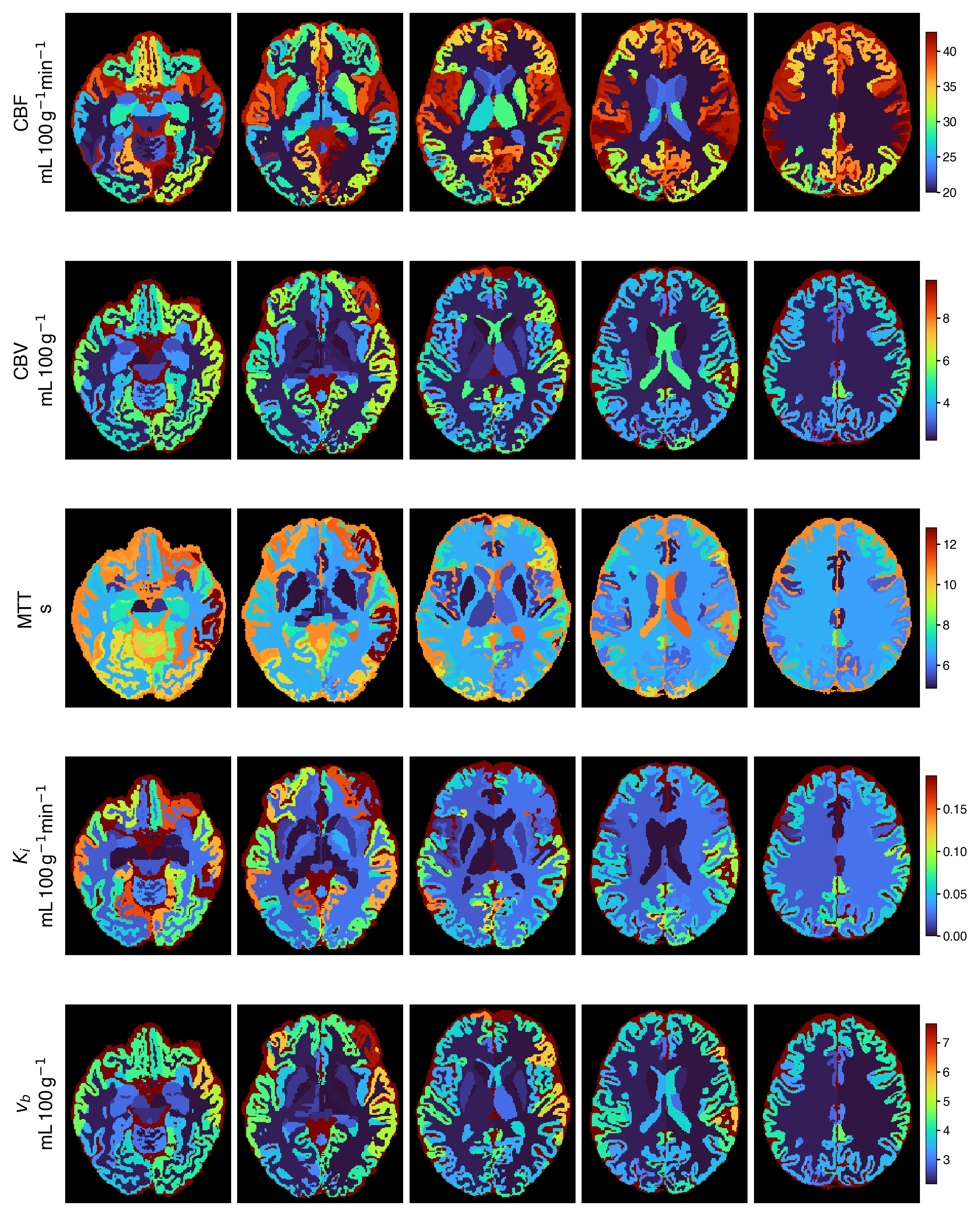
The default maps from a single automated run, namely Ki and vb from Patlak plus
CBF, MTT, and CBV from Tikhonov deconvolution, summarised per anatomical region,
alongside a diffusion metric. All come from one pbrain run with no manual
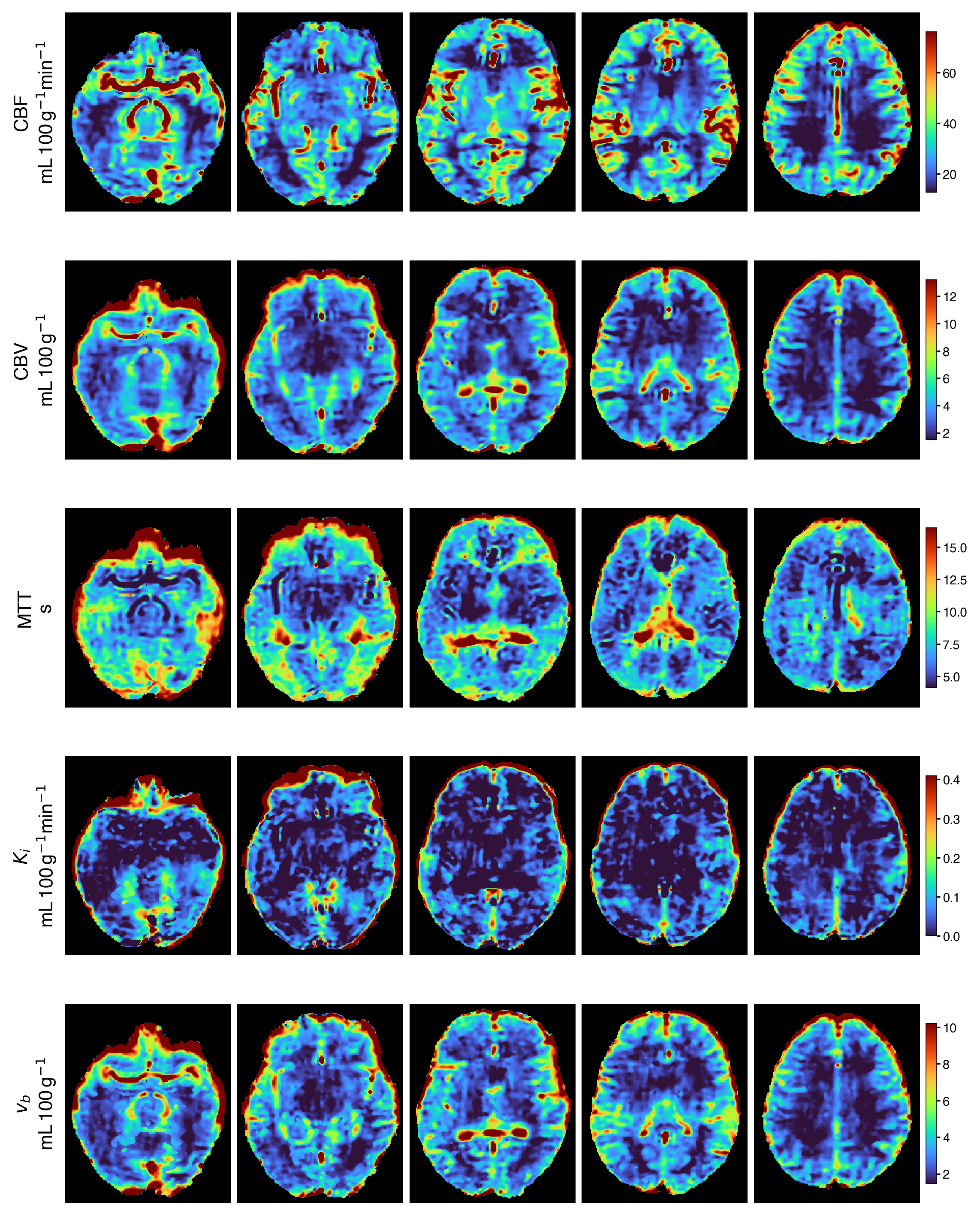
steps. The per-voxel view of the same maps is shown in the banner at the top of
this page.
Per-region, projected onto the SynthSeg parcellation
FA, fractional anisotropy, from the optional DTI diffusion track
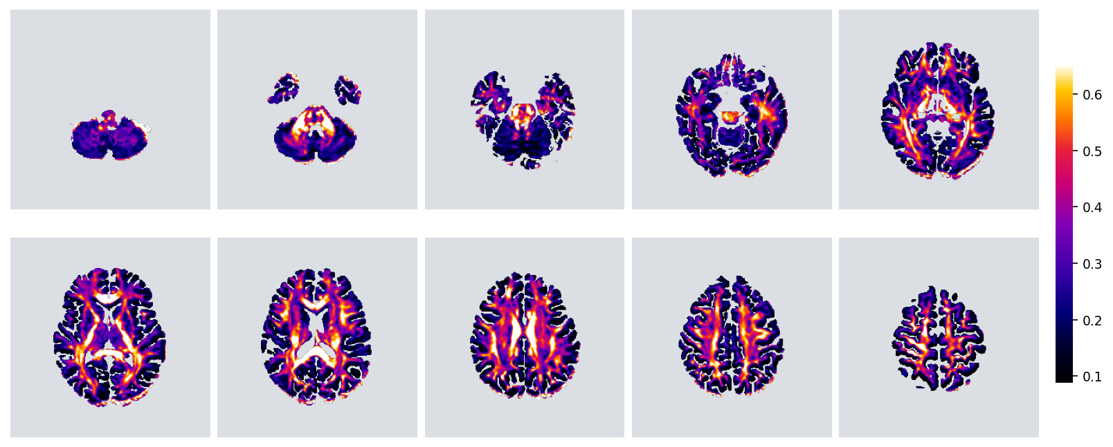
Every map is produced by the pipeline at voxel, tissue-class, and DKT-parcel level. See the paper for the full set and the quantitative validation.
Demo
python -m pbrain.demo --clean
This synthesises a small phantom, using no patient data, runs the entire
pipeline end-to-end, and writes parameter-map montages to demo/maps/. It is a
self-contained way to see the output format and confirm your install works.
Repository structure
pbrain/            the framework, everything lives here
  core/            Plugin/Stage contracts, discovery, Config, Pipeline, logging, QC
  io/              loaders (nifti/parrec/dicom/dwi) and output path schemes
  t1_m0/  aif/  tissue_roi/  signal_to_conc/  normalisation/    upstream stages
  models/          kinetic models          diffusion/   diffusion models
  aggregation/     voxel/region/parcel/slice rollups
  diagnostics/     per-model fit plots and the montage generator
  stages/          the pipeline steps (a discoverable, topologically ordered plug-point)
  cli/  demo/
docs/              ADDING_PLUGINS.md, ARCHITECTURE.md, mkdocs API reference
tests/             the test suite                validation/  cohort runners
Documentation
-
API reference. A rendered reference generated from the package docstrings, covering every public class, the plug-in contracts, the kinetic and diffusion models, the pipeline stages, and the QC functions. Build it locally with:
pip install "p-brain[docs]"
mkdocs build          # output in ./site/   (or run `mkdocs serve` for a live preview)
Entry points are
docs/index.mdand the contributor architecture overview. -
Extending the framework.
docs/ADDING_PLUGINS.mdhas copy-paste templates, anddocs/ARCHITECTURE.mdhas the full design rationale and output layout.
Citation
If p-Brain contributes to your work, please cite the accompanying paper (Tireli
et al.) and this repository. See
LICENSE for terms.
Release history Release notifications | RSS feed


Download files
Download the file for your platform. If you're not sure which to choose, learn more about installing packages.
Source Distribution
Built Distribution
Filter files by name, interpreter, ABI, and platform.
If you're not sure about the file name format, learn more about wheel file names.
Copy a direct link to the current filters
File details
Details for the file p_brain-3.0.7.tar.gz.
File metadata
- Download URL: p_brain-3.0.7.tar.gz
- Upload date:
- Size: 241.2 kB
- Tags: Source
- Uploaded using Trusted Publishing? No
- Uploaded via: twine/6.2.0 CPython/3.13.4
File hashes
| Algorithm | Hash digest | |
|---|---|---|
| SHA256 |
7f7edacf9121d2dc1ae8bfe19d16e49c51c64d543ab52e77a5027324dc778eca
|
|
| MD5 |
dfc6a788bc3ed7afdb0eb8254d5b01b6
|
|
| BLAKE2b-256 |
7fc26c881e3a7d5614a8fa45eb90e7390ad2736051261c79eaff14000b2d3978
|
File details
Details for the file p_brain-3.0.7-py3-none-any.whl.
File metadata
- Download URL: p_brain-3.0.7-py3-none-any.whl
- Upload date:
- Size: 280.9 kB
- Tags: Python 3
- Uploaded using Trusted Publishing? No
- Uploaded via: twine/6.2.0 CPython/3.13.4
File hashes
| Algorithm | Hash digest | |
|---|---|---|
| SHA256 |
e5242882d1697fd6e073369c91fca76c4d761921a3332a7129cb3e3ef78254f3
|
|
| MD5 |
d28ab98d0304f91ce244f55b32323530
|
|
| BLAKE2b-256 |
5ec0b4a641e8520f590321da72f5e265317eab04da80e594edbd009a9e2e40fb
|






