
PGraph: graphs for Python


Status & Project Health






Ecosystem & Dependencies





This pure-Python package provides classes for directed and undirected graphs: vertices connected by edges, with edge costs and path planning. Self-loops and parallel edges are permitted. Performance is good enough to support bundle adjustment, pose-graph SLAM and path planning over thousands of vertices.
Vertices can optionally be embedded: given a coordinate in a space of any
dimension. Edge costs are then computed from the vertex positions using a
distance metric (Euclidean, Manhattan, SE(2), or your own), the vertex nearest
a point can be found, A* uses the metric as its heuristic, and the graph can
be plotted, or exported with its layout preserved.
Installation
pip install pgraph-python
This needs Python 3.9 or later. The dependencies, NumPy, Matplotlib and Spatial Maths, are installed with it.
Examples
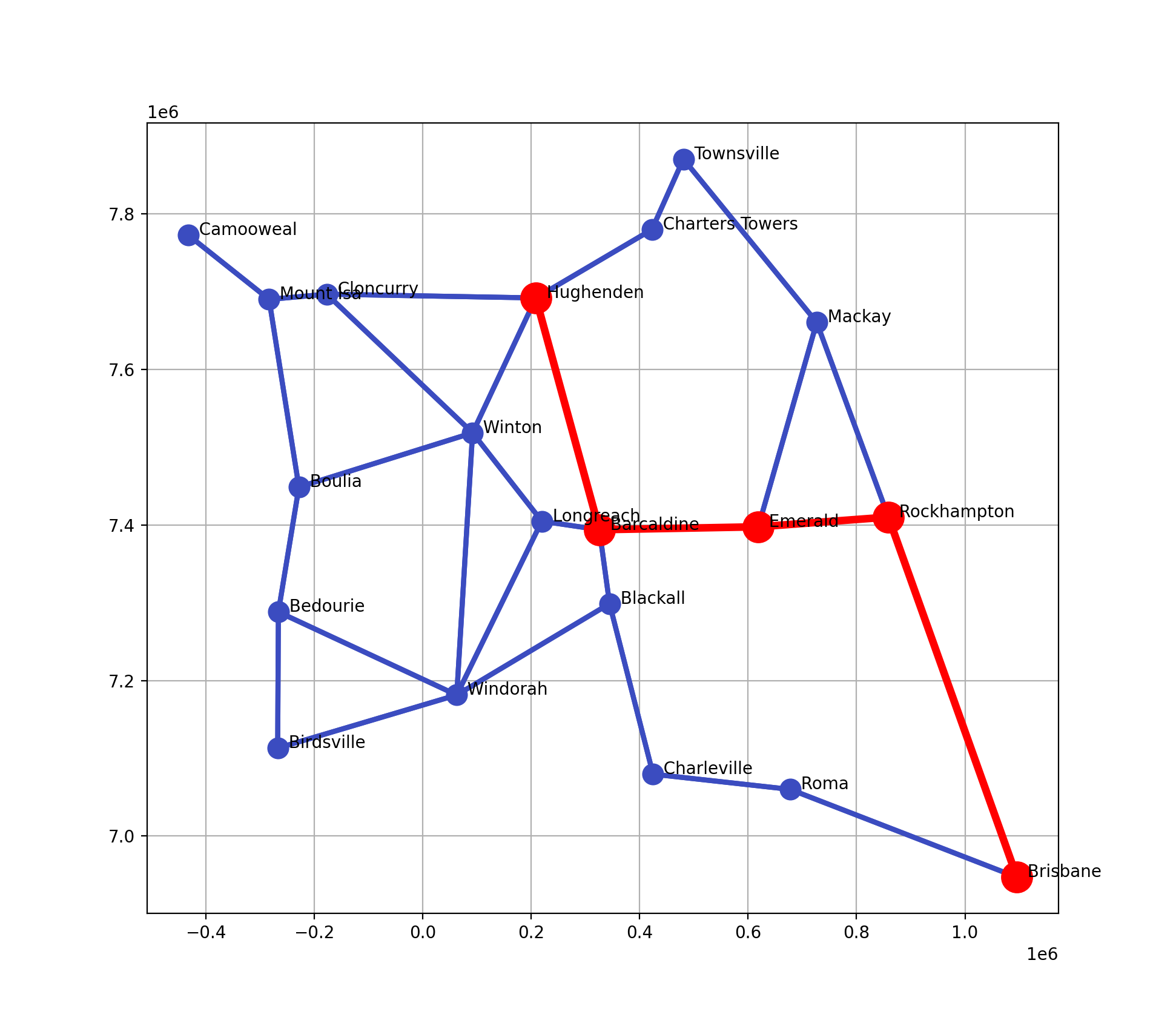
A small example: routing through towns in Queensland
from pgraph import UGraph
import json

# load the places and routes
with open('queensland.json', 'r') as f:
    data = json.load(f)

# build the graph
g = UGraph()
for name, info in data['places'].items():
    g.add_vertex(name=name, coord=info['utm'])
for route in data['routes']:
    g.add_edge(route['start'], route['end'], cost=route['distance'])

# plan a path from Hughenden to Brisbane
p, length, _ = g.path_Astar('Hughenden', 'Brisbane')
g.plot(block=False)  # plot it
g.highlight_path(p)  # overlay the path
The data file and the complete example are in the notebook examples/roads.ipynb.
A bigger example: routing through central London
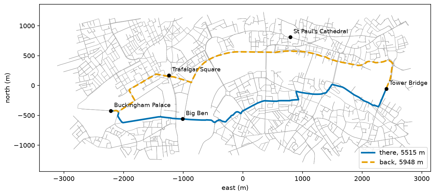
A directed graph of the road network of central London, taken from OpenStreetMap, and the shortest drive between Buckingham Palace and Tower Bridge, there (solid) and back (dashed). The two routes differ in length, 5,515 m and 5,948 m, because of the one-way streets. The notebook examples/london.ipynb builds the graph from the map data, keeps the part of it that can be driven around in, and plans with A*. This graph has over 4,000 vertices.
Map data © OpenStreetMap contributors, available under the Open Database License.
Using pgraph
Full details are given in the online documentation. For an AI assistant there is a short summary, llms.txt, and the complete documentation as one file, llms-full.txt.
Properties and methods of the graph
Graphs belong to the class UGraph or DGraph for undirected or directed graphs respectively. The graph is essentially a container for the vertices.
-
g.add_vertex()add a vertex -
g.nthe number of vertices -
gis an iterator over vertices, can be used asfor vertex in g: -
g[i]reference a vertex by its index or name
-
g.add_edge()connect two vertices -
g.edges()all edges in the graph -
g.plot()plots the vertices and edges -
g.ncthe number of graph components, 1 if fully connected -
g.component(c)the vertices in component numberc, numbered from 0 -
g.samecomponent(v1, v2)predicate for vertices belonging to the same component
-
g.path_BFS()breadth-first search, the path with the fewest edges -
g.path_UCS()uniform-cost search, the cheapest path -
g.path_Astar()A* search, the cheapest path using a heuristic
-
g.closest(point)the vertex nearest to a point -
g.near(point, radius)the vertices within a distance of a point -
g.within(box)the vertices inside a box -
g.subgraph(vertices)the part of the graph that those vertices induce, as a new graph -
g.coordinates()the vertex coordinates as a matrix, a column per vertex -
g.build_kdtree()an optional spatial index (needs scipy) that makesclosestandnearfaster on a large graph -
g.metricthe distance metric:"L2"(the default),"L1","SE2",SE2Metric(weight)that weights the angle of a pose, or a function of your own
-
g.adjacency()adjacency matrix -
g.laplacian()Laplacian matrix -
g.incidence()incidence matrix
-
g.copy()a deep copy; a graph can also be pickled -
g.export()write the graph as GraphViz DOT, Mermaid, GraphML, ELK, or an image (which needs GraphViz) -
g.validate()check that the graph's records agree with each other
Properties and methods of a vertex
Vertices are instances of the class Vertex, for both undirected and directed graphs.
v.coordthe coordinate vector for embedded graph (optional)v.namethe name of the vertex (optional)v.labelthe number of the component that the vertex belongs tov.adjacent()is a list of the adjacent vertices (neighbours()andneighbors()are the same)
Vertices can be named and referenced by name.
Properties and methods of an edge
Edges are instances of the class Edge.
Each edge references a pair of vertices, the graph lists all of its edges in g.edges(), and the vertices reference the edges.
e.costcost of edge for planning methodse.next(v)vertex on edgeethat is notve.v1,e.v2the two vertices that define the edgee
Modifying a graph
g.remove_vertex(v)orv.remove()remove vertexvg.remove_edge(e)ore.remove()remove edgee
Subclassing pgraph classes
Consider a user class Foo that we would like to connect using a graph overlay, i.e.
instances of Foo become vertices in a graph.
- Have it subclass
Vertex - Then place instances of
Foointo the graph usingadd_vertexand create edges as required
from pgraph import UGraph, Vertex

class Foo(Vertex):
    # foo stuff goes here
    def say_hi(self):
        print(f"hi from {self.name}")

f1 = Foo(name="f1")
f2 = Foo(name="f2")

g = UGraph() # create a new undirected graph
g.add_vertex(f1)
g.add_vertex(f2)

f1.connect(f2, cost=3)
for f in f1.adjacent():
    f.say_hi()  # say hi to the neighbours
Or tell the graph which classes to make, with UGraph(vertex_class=Foo, edge_class=Bar), and g.add_vertex() and g.add_edge() create instances of them, so they never need to be constructed by hand.
Performance
Timings of the key operations on random geometric graphs, each vertex joined to its 4 nearest neighbours, of 100, 1,000 and 10,000 vertices, measured with examples/benchmark.py on an Apple M4 with Python 3.12 and NumPy 2.5. The path times are the median of 10 random start and goal pairs. The last column is the exponent b in time ∝ Nb between the smallest and the largest graph for the quantity shown, so 0 is constant, 1 is linear and 2 is quadratic. The adjacency, Laplacian and incidence matrices are dense, so they are only formed up to 1,000 vertices.
Undirected graphs
| Operation | per | N=100 | N=1,000 | N=10,000 | growth exponent |
|---|---|---|---|---|---|
| add a vertex | µs / vertex | 0.83 | 0.877 | 0.896 | 0.0 |
| add an edge (cost from the metric) | µs / edge | 1.54 | 1.64 | 1.72 | 0.0 |
| copy the graph | ms | 0.819 | 8.36 | 155 | 1.1 |
| pickle and unpickle the graph | ms | 0.462 | 4.87 | 90.4 | 1.1 |
| number of components, after a change | ms | 0.03 | 0.338 | 4.09 | 1.1 |
| number of components, unchanged | µs | 0.083 | 0.083 | 0.083 | 0.0 |
| remove a vertex | µs | 6.67 | 18 | 74.2 | 0.5 |
| closest vertex to a point | µs / query | 73.7 | 734 | 7,069 | 1.0 |
| adjacency matrix | ms | 0.11 | 1.53 | – | 1.1 |
| Laplacian matrix | ms | 0.122 | 2.93 | – | 1.4 |
| incidence matrix | ms | 0.0568 | 1.37 | – | 1.4 |
| path, breadth-first | ms / query | 0.0385 | 0.32 | 4.77 | 1.0 |
| path, uniform cost | ms / query | 0.0848 | 0.865 | 10.4 | 1.0 |
| path, A* | ms / query | 0.0521 | 0.306 | 2.71 | 0.9 |
Directed graphs
| Operation | per | N=100 | N=1,000 | N=10,000 | growth exponent |
|---|---|---|---|---|---|
| add a vertex | µs / vertex | 0.769 | 0.797 | 0.856 | 0.0 |
| add an edge (cost from the metric) | µs / edge | 1.55 | 1.66 | 1.7 | 0.0 |
| copy the graph | ms | 1.14 | 12.6 | 215 | 1.1 |
| pickle and unpickle the graph | ms | 0.586 | 6.88 | 169 | 1.2 |
| number of components, after a change | ms | 0.0419 | 0.49 | 6.35 | 1.1 |
| number of components, unchanged | µs | 0.083 | 0.083 | 0.083 | 0.0 |
| remove a vertex | µs | 8.33 | 24 | 74.7 | 0.5 |
| closest vertex to a point | µs / query | 69.4 | 703 | 7,242 | 1.0 |
| adjacency matrix | ms | 0.0816 | 1.27 | – | 1.2 |
| Laplacian matrix | ms | 0.093 | 2.81 | – | 1.5 |
| incidence matrix | ms | 0.0885 | 2.23 | – | 1.4 |
| path, breadth-first | ms / query | 0.0332 | 0.412 | 4.36 | 1.1 |
| path, uniform cost | ms / query | 0.0607 | 0.944 | 8.26 | 1.1 |
| path, A* | ms / query | 0.0487 | 0.728 | 3.57 | 0.9 |
History
This is a re-engineered version of PGraph.m which ships as part of the Spatial Math Toolbox for MATLAB. That class was used to support bundle adjustment, pose-graph SLAM and various planners such as PRM, RRT and Lattice.
The Python version was designed from the start to work with directed and undirected graphs, whereas directed graphs were a late addition to the MATLAB version. Semantics are similar but not identical. In particular the use of subclassing rather than references to user data is encouraged.
1 maintainer

Metadata
1 maintainer
Release files for pgraph-python 1.0.0
For a detailed explanation of source distributions (sdists) and built distributions (wheels), please see the package formats documentation.
Source distribution (sdist)
| File | Size | Uploaded | |
|---|---|---|---|
| pgraph_python-1.0.0.tar.gz | 2.0 MB | Details |
Built distribution (wheel)
| File | Interpreter | ABI | Platform | Reset |
|---|---|---|---|---|
| pgraph_python-1.0.0-py3-none-any.whl | Python 3 | none | any | Details |
Total release size: 2.1 MB
Release files / pgraph_python-1.0.0.tar.gz
| Download URL | pgraph_python-1.0.0.tar.gz |
|---|---|
| Size | 2.0 MB |
| Tags | Source |
|
SHA-256 checksum How to use checksums |
f5bc1c3ecc3c11cc3619e7a8bd82ad1bf17bf3888ffb7c06b1709cd010f7d407
|
|
BLAKE2b-256 checksum How to use checksums |
86146e56991f3a16c0eb7645064757689b7ca26c46f833c6003673c113a27ef4
|
| Upload date | |
|
Uploaded using Trusted Publishing? What is trusted publishing? |
Yes |
| Uploaded via |
twine/7.0.0 CPython/3.13.14
|
Provenance
Provenance describes where a file came from. On PyPI, provenance is shared via attestations, which provide a verifiable record of the build or publishing details. View details, limitations and caveats.


PyPI Publish Attestation
PyPI verified that this artifact, at this checksum, originated from the publisher listed below.
Signed by GitHub Actions, verified by PyPI on Oct 13, 2026.
Transparency logRelease files / pgraph_python-1.0.0-py3-none-any.whl
| Download URL | pgraph_python-1.0.0-py3-none-any.whl |
|---|---|
| Size | 61.3 kB |
| Tags | Python 3 |
|
SHA-256 checksum How to use checksums |
0f5fe00ea05473e8eee70861a004e4e2541ba3424e14213d9ec249bbc21f69cf
|
|
BLAKE2b-256 checksum How to use checksums |
767cfaef5a489310236f43f0553d6982278e6e6a859f2a6bbf3c7cad2abe16ee
|
| Upload date | |
|
Uploaded using Trusted Publishing? What is trusted publishing? |
Yes |
| Uploaded via |
twine/7.0.0 CPython/3.13.14
|
Provenance
Provenance describes where a file came from. On PyPI, provenance is shared via attestations, which provide a verifiable record of the build or publishing details. View details, limitations and caveats.
PyPI Publish Attestation
PyPI verified that this artifact, at this checksum, originated from the publisher listed below.
Signed by GitHub Actions, verified by PyPI on Oct 13, 2026.
Transparency log













