
Tools for phase autocoherence analysis with dynamic windowing methods

Project description
phaseco
A Python package for phase autocoherence analysis with dynamic windowing methods.
Installation
You can install phaseco directly from PyPI:
pip install phaseco
or from the latest GitHub source:
pip install git+https://github.com/seththepeacock/phaseco.git
Links
Overview
phaseco quantifies the self-coherence in phase of the oscillations in a signal as a function of frequency.
It includes functions for:
- Estimating autocoherence, a spectrum representing stability in phase evolution over a fixed reference time as a function of frequency
- Building colossograms (from coherence-loss-o-gram) for visualization of the decay in autocoherence with increasing reference time
- Extracting time constants representing this decay for a given frequency
- Implementing dynamic windowing methods to deal with issues associated with the time-frequency tradeoff
Example use
Import the package:
import phaseco as pc
Define your waveform and its samplerate:
wf = []
fs = 44100
The heart of the method is a short-time Fourier transform (STFT) to obtain magnitude and phase estimates as a function of time and frequency. Define $\tau$, the length of each segment in the STFT which (along with the window shape) sets the bandwidth of the effective filter in the filterbank interpretation of the STFT.
tau_s = 0.0745 # 74.5ms corresponds to an effective filter half-power bandwidth of ~50Hz for a flattop window
tau = int(round(tau_s*fs)) # Convert to samples. If this isn't a power of 2, the segments will be zero padded for FFT efficiency.
Another STFT parameter is the hop length; smaller hops allow for more information to be extracted from a given signal length at the cost of longer computation time. The default is $\tau/2$ (50% overlap).
hop_s = 0.01 # 10ms
hop = int(round(hop_s*fs)) # Convert to samples
Using the phase estimates, we will quantify the consistency of each frequency component's phase evolution over the reference time $\xi$.
xi_s = 0.02 # 20ms
xi = int(round(xi_s*fs)) # Convert to samples
Determine whether to use 'power-weights'. pw=False uses only phases from the STFT while True uses magnitude as well by weighting each instance of phase evolution by the product of magnitudes in each segment and its $\xi$-advanced partner.
pw = False
Calculate the autocoherence for a single reference time $\xi$:
f, ac = pc.get_autocoherence(wf, fs, xi, pw, tau, hop=hop) # Frequency array, autocoherence array
We can also calculate how the autocoherence decays over increasing reference time $\xi$. Set the array of these reference times by determining the min, max, and grid spacing (in seconds).
xis = {'xi_min_s':0.001, 'xi_max_s':0.100, 'delta_xi_s':0.001} # 1ms to 100ms in 1ms steps
Note that all frequency bins will show high autocoherence for small reference times relative to window length (i.e. $\xi\ll\tau$).
- This can be understood directly; if $\xi\ll\tau$ each window will contain almost the same set of samples as its $\xi$-advanced partner. Therefore even for random noise, the phase evolution over short $\xi$ (that is, the difference in phase at a given point in time $\phi$ to one $\xi$ samples later $\phi_\xi$) will always be consistently near $\phi_\xi-\phi= \omega\xi$ leading to spuriously high autocoherence.
- This can also be understood as a consequence of the time-frequency tradeoff. Large $\tau$ means the effective filters in the STFT are very narrow; this localization in frequency smears timing information over small timescales $\xi$ so that the phase evolution is always approximately consistent/coherent.
Moreover, for a fixed 'static' window shape of fixed length $\tau$, all frequencies' autocoherence will decay in nearly the same way as $\xi\rightarrow\tau$. This makes it difficult to extract information from this decay at a particular frequency of interest.
To address this, we implement dynamic windowing methods which result in a wider effective filter (broad localization in frequency) for low $\xi$ (when tight localization in time is needed); see "Overview of Windowing Methods."
win_meth = {"method": "rho", "win_type": "flattop", "rho": 1.0}
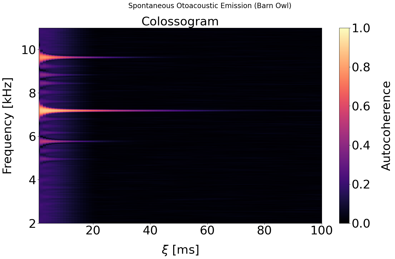
We can then calculate a "colossogram" (from coherence-loss-o-gram) to track how the autocoherence decays as a function of $\xi$ for all frequency components.
cgram_dict = pc.get_colossogram(wf, fs, xis, pw, tau, hop=hop, win_meth=win_meth)
This dictionary contains the $\xi$ array, frequency array, and autocoherence values themselves:
xis_s = cgram_dict['xis_s']
f = cgram_dict['f']
colossogram = cgram_dict['colossogram']
However, the dictionary can be directly passed into a plotting function (based on matplotlib.pyplot):
plt.figure()
pc.plot_colossogram(cgram_dict)
plt.show()
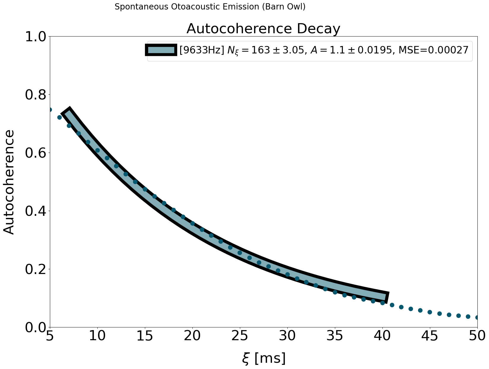
Finally, we can estimate a (nondimensionalized) time constant N_xi representing the rate of decay in autocoherence for a given frequency f0. This is done by fitting an exponential decay $Ae^{t(\xi)/T_\xi}$, where $t(\xi)=\xi/f_s$. The time constant $T_\xi$ is then nondimensionalized as $N_\xi = T_\xi \cdot f_0$, representing the number of cycles a sinusoid at frequency $f_0$ would pass through in $T_\xi$ seconds.
f0 = 1000 # in Hz
N_xi, decay_dict = pc.get_N_xi(cgram_dict, f0)
Again, we can plot this decay and its exponential fit by passing in the dictionary to a built-in plotting function:
plt.figure()
pc.plot_N_xi(decay_dict)
plt.show()
Overview of Windowing Methods
'static'— Fixed window defined bywin_type.'rho'— Dynamically increases the standard deviation $\sigma$ of a (truncated) Gaussian window $w_\xi[n]$ with $\xi$ so the spurious expected autocoherence for white noise (due to shared samples between a window and its $\xi$-advanced partner) remains low. The final window used is $w[n]=w_\xi[n] \cdot w_0[n]$ where $w_0[n]$ is the fixed "asymptotic window" determined bywin_type.- Specifically, $\sigma$ is set such that the Gaussian's full width half maximum (FWHM) is
rho * xi. - Both $w_\xi[n]$ and $w_0[n]$ have fixed length $\tau$.
- Specifically, $\sigma$ is set such that the Gaussian's full width half maximum (FWHM) is
'zeta'— Dynamically sets window length so the (power-weighted) expected autocoherence for white noise remains fixed atzeta. Once the reference time $\xi$ is large enough that dynamically chosen window length would exceed the originally chosen $\tau$ parameter, it remains fixed at that $\tau$ for all larger $\xi$.
Implementing windowing methods
The win_meth dictionary defines dynamic windowing methods used in several phaseco functions.
Structure
win_meth = {
    "method": "rho",
    "win_type": "flattop",
    "rho": 1.0,
}
Keys
| Key | Type | Description |
|---|---|---|
method |
str | Windowing method: 'static', 'rho', or 'zeta'. |
win_type |
str or tuple | Window type (passed to scipy.signal.get_window()). |
rho |
float | FWHM multiplier for Gaussian window (used in 'rho' method). |
zeta |
float | Controls allowable spurious autocoherence in 'zeta' method. |
snapping_rhortle |
bool | When True and method='rho', switches to boxcar for all $\xi>\tau$. |
More examples
Self-contained example scripts are available here. One demonstrates most phaseco functions by analyzing a sinsusoid with brownian phase noise; another displays how zeta windowing pins the observed (power-weighted) autocoherence for white noise at $\approx \zeta$.
More info
For more details on each function, see the documented funcs.py file in the source code.
Release history Release notifications | RSS feed


Download files
Download the file for your platform. If you're not sure which to choose, learn more about installing packages.
Source Distribution
Built Distribution
Filter files by name, interpreter, ABI, and platform.
If you're not sure about the file name format, learn more about wheel file names.
Copy a direct link to the current filters
File details
Details for the file phaseco-0.1.0.tar.gz.
File metadata
- Download URL: phaseco-0.1.0.tar.gz
- Upload date:
- Size: 328.0 kB
- Tags: Source
- Uploaded using Trusted Publishing? No
- Uploaded via: twine/6.1.0 CPython/3.13.7
File hashes
| Algorithm | Hash digest | |
|---|---|---|
| SHA256 |
dc09c3c342bbaa78c3d22307527e3f29332b1a863c0ea398d8ea6c206cc93e4b
|
|
| MD5 |
0d42607980ad89746046fcb3f75141ce
|
|
| BLAKE2b-256 |
25d8eee80a1ba4d2683208be343164b78a3f5e1d0e8b3717e030daf859b63000
|
File details
Details for the file phaseco-0.1.0-py3-none-any.whl.
File metadata
- Download URL: phaseco-0.1.0-py3-none-any.whl
- Upload date:
- Size: 326.9 kB
- Tags: Python 3
- Uploaded using Trusted Publishing? No
- Uploaded via: twine/6.1.0 CPython/3.13.7
File hashes
| Algorithm | Hash digest | |
|---|---|---|
| SHA256 |
6efdca9ca1f275c102388ddc54f192c58bce87df60b9ef86bb3edfbb72cae633
|
|
| MD5 |
85ab538381e05658a62b583fd8ae25d4
|
|
| BLAKE2b-256 |
21180aae3acb032ce9a05b797ffddbada8c28cf1cea05d85ec41ff25f2888c55
|






