
plotly-calheatmap
A continuation of plotly-calplot by Bruno Rocha Silva, which is no longer actively maintained.
This project picks up where plotly-calplot left off, providing an interactive calendar heatmap built with Plotly — similar to the contribution graphs on GitHub and GitLab profile pages.
Features
- Interactive calendar heatmaps built with Plotly
- Multi-layer heatmap — overlay multiple DataFrames on one calendar with distinct color gradients per source; overlap days are summed and shown in a third colorscale (
layersparameter) - Dataset swap — switch between multiple metrics via dropdown without regenerating the graph (
datasetsparameter) - Built-in aggregation — pass raw event data with
agg="sum"|"mean"|"count"|"max"instead of pre-aggregating - Logarithmic color scale —
log_scale=Trueapplieslog(1+x)so extreme values don't wash out the heatmap - Custom time groupings —
grouping="quarter"|"bimester"|"semester"draws separator lines and replaces axis labels - Vertical orientation — render months as rows with
vertical=True - Hourly heatmap —
hourly_calheatmap()for hour × day grids per month - Skip empty years —
skip_empty_years=Trueexcludes years with no data - Replace NaNs with zeros —
replace_nans_with_zeros=Truedisplays empty dates as 0 - Top & bottom border lines —
top_bottom_lines=Truedraws horizontal lines enclosing each month - Month gap spacing — extra visual separation between months via
month_gap - Custom week start day —
week_start="sunday"or"saturday"to change the first day of the week (default:"monday") - Wall-calendar layout —
layout="calendar"renders a grid of mini-calendars with days as columns and weeks as rows - Multi-year support with independent tick configurations per subplot
- Year navigation buttons (
navigation=True) - Localization support (
localeparameter) for month and day names (e.g.pt_BR,es,fr) - Customizable hovertemplate with friendly
{placeholder}syntax andcustomdatacolumns - Smart colorscales — pass a
colorslist andscale_type("linear","quantile","quantize","diverging","categorical") for automatic interval computation - Cell annotations —
annotations=Trueorannotations_fmt="%{z:.0f}"displays values/labels inside each cell - Zero-value distinction —
zero_colorgives 0-value cells a dedicated color while missing data stays transparent - Missing-data styling —
nan_colorassigns a dedicated color to NaN/missing cells, distinguishing them from zero-value cells - Responsive / auto-sizing — all chart types adapt width to the container automatically; height is computed from the data (overridable via
total_heightandwidth) - Fully customizable colorscales (including custom lists)
- Month separator lines, configurable month label placement, and color scale with label/ticks
- Flexible layout options:
gap,margin,font_*,paper_bgcolor,plot_bgcolor, etc.
Documentation
For the full API reference (all parameters for calheatmap() and hourly_calheatmap()), see docs/API.md.
Installation
pip install plotly-calheatmap
Quick Start
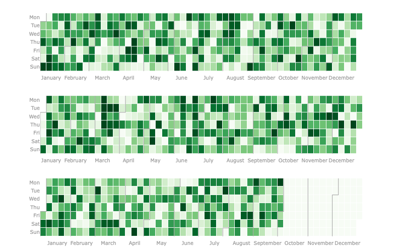
from plotly_calheatmap import calheatmap

fig = calheatmap(df, x="date", y="value")
fig.show()
Built-in Aggregation
Pass raw (non-aggregated) event data directly — duplicate dates are grouped and aggregated automatically:
from plotly_calheatmap import calheatmap

# df has multiple rows per date (e.g. individual transactions)
fig = calheatmap(df, x="date", y="amount", agg="sum")
fig.show()
Supported functions: "sum", "mean", "count", "max".
Vertical Orientation
fig = calheatmap(df, x="date", y="value", vertical=True, month_gap=1)
Dataset Swap
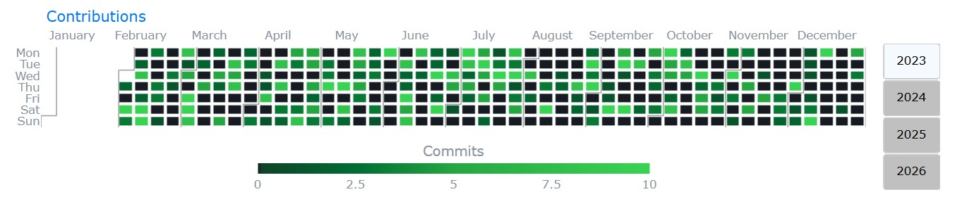
Switch between multiple metrics on the same graph via a dropdown menu. Each dataset can have its own colorscale, value range, and legend title. Works with both calheatmap() and hourly_calheatmap(), alongside year navigation.
fig = calheatmap(
    data=df,
    x="date",
    y="sales",
    datasets={
        "Sales": {
            "y": "sales",
            "colorscale": "greens",
            "showscale": "Sales ($)",
            "cmap_min": 0,
        },
        "Activity": {
            "y": "activity",
            "colorscale": "blues",
            "showscale": "Activity (hours)",
        },
    },
    navigation=True,
)
Logarithmic Color Scale
When a few extreme values wash out the rest of the heatmap, use log_scale=True to apply log(1+x) to the color mapping. Hover text still shows original values.
fig = calheatmap(df, x="date", y="value", log_scale=True)
Smart Colorscales & Zero Distinction
Instead of manually defining colorscale intervals, pass a list of colors and let the library compute the positions automatically:
# Old way (manual positions)
colorscale=[[0.0, "#161b22"], [0.01, "#0e4429"], [0.25, "#006d32"], [1.0, "#39d353"]]

# New way (automatic)
colors=["#0e4429", "#006d32", "#26a641", "#39d353"],
zero_color="#161b22"  # dedicated color for value 0
Scale types control how colors are distributed:
# linear (default): colors evenly spaced across data range
fig = calheatmap(df, x="date", y="value",
    colors=["#edf8e9", "#bae4b3", "#74c476", "#31a354", "#006d2c"])

# quantile: each color covers equal number of data points (good for skewed data)
fig = calheatmap(df, x="date", y="value",
    colors=["#edf8e9", "#bae4b3", "#74c476", "#006d2c"],
    scale_type="quantile")

# quantize: data range split into equal mathematical intervals
fig = calheatmap(df, x="date", y="value",
    colors=["#edf8e9", "#bae4b3", "#74c476", "#006d2c"],
    scale_type="quantize")

# diverging: two gradients meeting at a pivot point
fig = calheatmap(df, x="date", y="temp",
    colors=["#2166ac", "#f7f7f7", "#b2182b"],
    scale_type="diverging", pivot=20, symmetric=True)

# categorical: user-defined bins with explicit color per range
fig = calheatmap(df, x="date", y="value",
    scale_type="categorical",
    bins=[(0, 0, "gray"), (1, 3, "lightgreen"), (4, float("inf"), "darkgreen")])
Zero-value distinction — give cells with value 0 a dedicated color, separate from missing data (which stays transparent):
fig = calheatmap(df, x="date", y="commits",
    colors=["#0e4429", "#006d32", "#26a641", "#39d353"],
    zero_color="#161b22")
Missing-data styling — give NaN/missing cells a visible color instead of leaving them transparent:
fig = calheatmap(df, x="date", y="commits",
    colors=["#0e4429", "#006d32", "#26a641", "#39d353"],
    zero_color="#161b22",
    nan_color="#0d1117")
All new parameters also work inside the datasets dict for per-metric configuration.
Cell Annotations
Display values or labels inside each cell:
# Show integer values inside cells
fig = calheatmap(df, x="date", y="score",
    annotations=True, annotations_fmt="%{z:.0f}",
    gap=4, total_height=280)

# Simple boolean — shows raw z values
fig = calheatmap(df, x="date", y="score", annotations=True)

Custom Time Groupings
Draw thicker separator lines at quarter, bimester, or semester boundaries and replace axis labels with group names:
fig = calheatmap(df, x="date", y="value", grouping="quarter", month_lines=True)

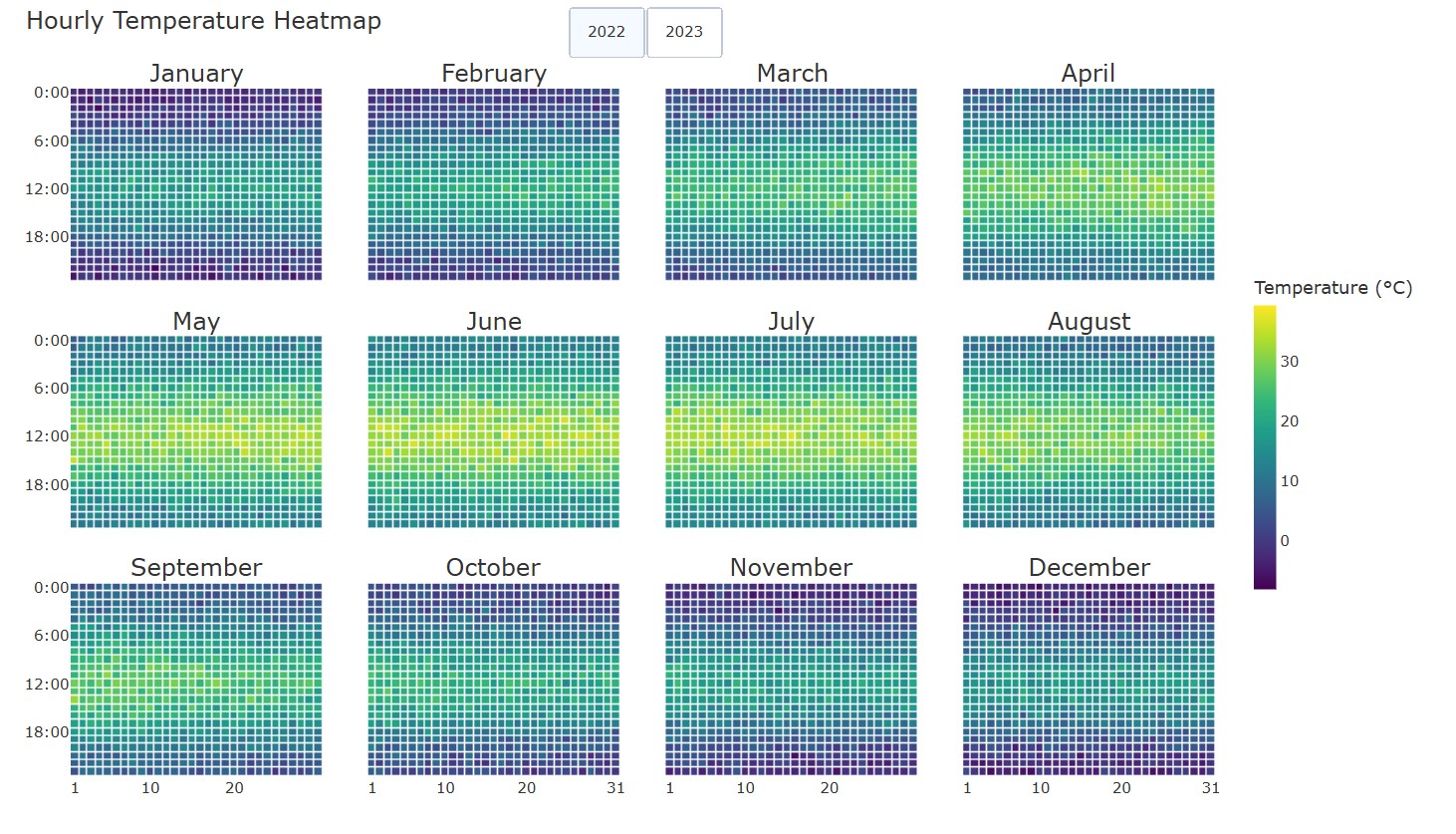
Hourly Heatmap
from plotly_calheatmap import hourly_calheatmap

fig = hourly_calheatmap(df, x="datetime_col", y="value")
fig.show()
Skip Empty Years & Replace NaNs
fig = calheatmap(df, x="date", y="value", skip_empty_years=True, replace_nans_with_zeros=True)
Border Lines
Fully enclose each month by combining month_lines with top_bottom_lines:
fig = calheatmap(df, x="date", y="value", month_lines=True, top_bottom_lines=True)
Custom Week Start Day
Choose which day the week starts on — "monday" (default, ISO 8601), "sunday" (US convention), or "saturday":
fig = calheatmap(df, x="date", y="value", week_start="sunday")
Multi-Layer Heatmap
Overlay two (or more) DataFrames on one calendar. Each source gets its own color gradient; days present in both are summed and shown with a third colorscale:
fig = calheatmap(
    layers=[
        {"data": revenue,  "x": "date", "y": "value", "colorscale": "blues",  "name": "Revenue"},
        {"data": expenses, "x": "date", "y": "value", "colorscale": "reds",   "name": "Expenses"},
    ],
    overlap_colorscale="greens",
)
Hover shows per-source values and the combined total for overlap days.

Wall-Calendar Layout
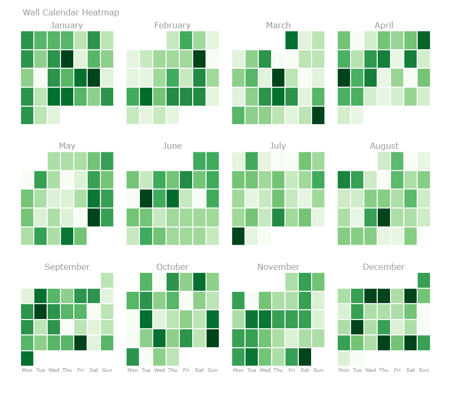
Render a grid of mini-calendars (one per month), each looking like a standard wall calendar with days-of-week as columns and weeks as rows:
fig = calheatmap(df, x="date", y="value", layout="calendar", cols=4)
Credits
This project is based on the original work by Bruno Rocha Silva — plotly-calplot.
1 maintainer

Metadata
1 maintainer
Release files for plotly-calheatmap 0.5
For a detailed explanation of source distributions (sdists) and built distributions (wheels), please see the package formats documentation.
Source distribution (sdist)
| File | Size | Uploaded | |
|---|---|---|---|
| plotly_calheatmap-0.5.tar.gz | 41.3 kB | Details |
Built distribution (wheel)
| File | Interpreter | ABI | Platform | Reset |
|---|---|---|---|---|
| plotly_calheatmap-0.5-py3-none-any.whl | Python 3 | none | any | Details |
Total release size: 85.3 kB
Release files / plotly_calheatmap-0.5.tar.gz
| Download URL | plotly_calheatmap-0.5.tar.gz |
|---|---|
| Size | 41.3 kB |
| Tags | Source |
|
SHA-256 checksum How to use checksums |
da894d9f288cd3b84d21b09cc597ca42f917c8a3492f679ee77af83f2bcd82e1
|
|
BLAKE2b-256 checksum How to use checksums |
7a9e49e3eea721f5d17233cfb97cfc601800f49457c0a0f03e025ce63e94751c
|
| Upload date | |
|
Uploaded using Trusted Publishing? What is trusted publishing? |
Yes |
| Uploaded via |
twine/6.1.0 CPython/3.13.7
|
Provenance
Provenance describes where a file came from. On PyPI, provenance is shared via attestations, which provide a verifiable record of the build or publishing details. View details, limitations and caveats.


PyPI Publish Attestation
PyPI verified that this artifact, at this checksum, originated from the publisher listed below.
Signed by GitHub Actions, verified by PyPI on Jan 31, 2026.
Transparency logRelease files / plotly_calheatmap-0.5-py3-none-any.whl
| Download URL | plotly_calheatmap-0.5-py3-none-any.whl |
|---|---|
| Size | 44.0 kB |
| Tags | Python 3 |
|
SHA-256 checksum How to use checksums |
752e251c188ee8b46f04776d7cdfef96c6fa7c54f59c74df2c9c828b8965d245
|
|
BLAKE2b-256 checksum How to use checksums |
9da80302812bed2c4d65bb1466d91cba90f48f817f74f660c4bb7ca40240d555
|
| Upload date | |
|
Uploaded using Trusted Publishing? What is trusted publishing? |
Yes |
| Uploaded via |
twine/6.1.0 CPython/3.13.7
|
Provenance
Provenance describes where a file came from. On PyPI, provenance is shared via attestations, which provide a verifiable record of the build or publishing details. View details, limitations and caveats.
PyPI Publish Attestation
PyPI verified that this artifact, at this checksum, originated from the publisher listed below.
Signed by GitHub Actions, verified by PyPI on Jan 31, 2026.
Transparency log













