
PlanetaRY spanGLES: general photometry of planets, rings and shadows

Project description
Pryngles
PlanetaRY spaNGLES











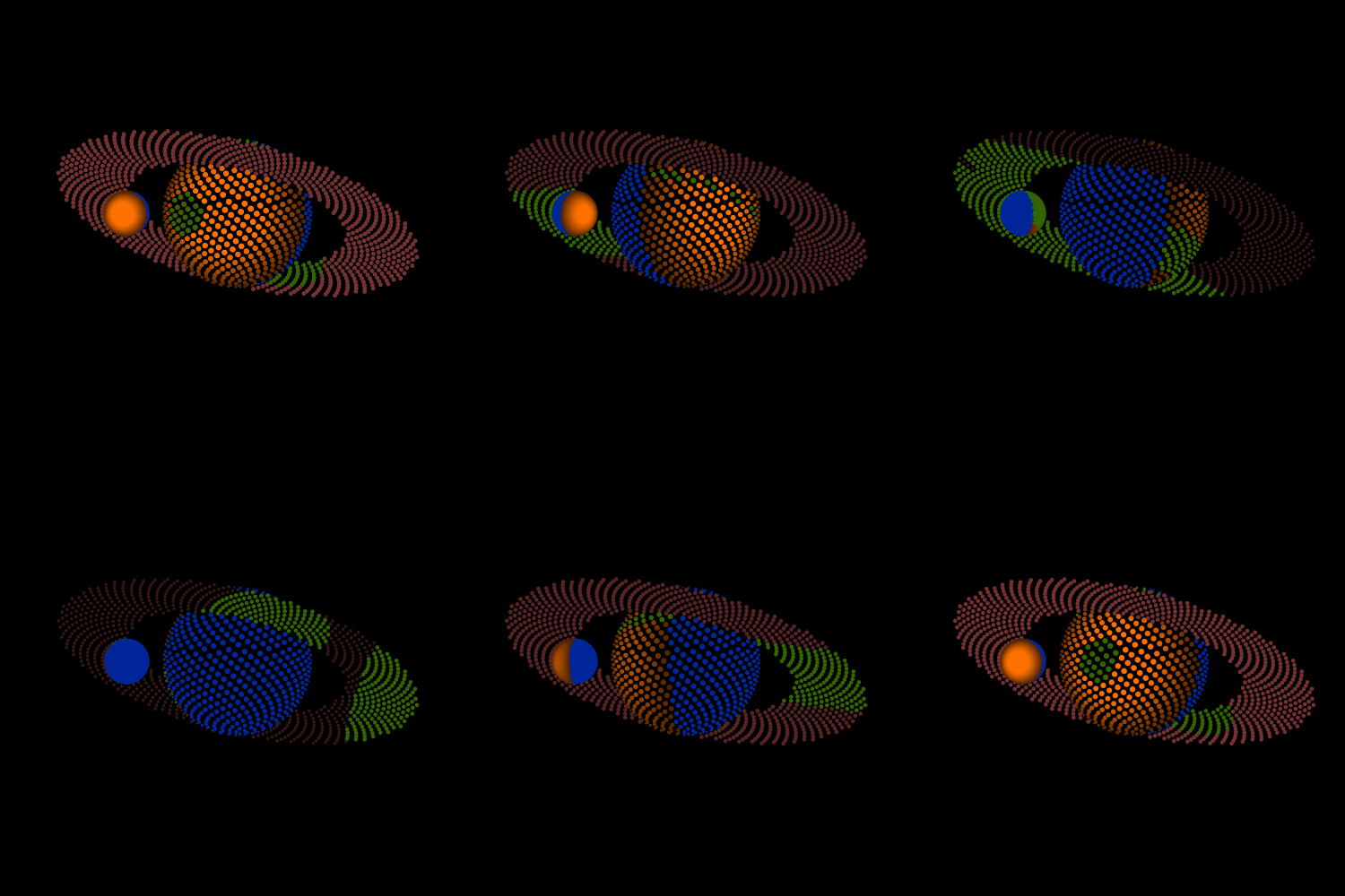
Pryngles is a Python package intended to produce useful
visualizations of the geometric configuration of a ringed exoplanet
(an exoplanet with a ring or exoring for short) and more importantly
to calculate the light curve produced by this kind of planets. The
model behind the package has been developed in an effort to predict
the signatures that exorings may produce not only in the light curve
of transiting exoplanets (a problem that has been extensively studied)
but also in the light of stars having non-transiting exoplanets (the
bright side of the light curve).
For the science behind the model please refer to the following papers:
Veenstra, A. K., Zuluaga, J. I., Alvarado-Montes, J. A., Sucerquia, M., & Stam, D. M. (2025), A general polarimetric model for transiting and nontransiting ringed exoplanets, Astronomy & Astrophysics, 693, A310, doi:10.1051/0004-6361/202347194, A&A article, PDF (repo).
Zuluaga, J.I., Sucerquia, M. & Alvarado-Montes, J.A. (2022), The bright side of the light curve: a general photometric model for non-transiting exorings, Astronomy and Computing 40 (2022) 100623, doi:10.1016/j.ascom.2022.100623, arXiv:2207.08636, PDF (repo).
Sucerquia, M., Alvarado-Montes, J. A., Zuluaga, J. I., Montesinos, M., & Bayo, A. (2020), Scattered light may reveal the existence of ringed exoplanets. Monthly Notices of the Royal Astronomical Society: Letters, 496(1), L85-L90, doi:10.1093/mnrasl/slaa080, journal article, PDF (repo).
Citation
If you use pryngles in your research, please cite the relevant paper(s):
@article{ZuluagaEtAl2025AA,
  author  = {Veenstra, Allard K. and Zuluaga, Jorge I. and Alvarado-Montes, Jaime A. and Sucerquia, Mario and Stam, Daphne M.},
  title   = {A general polarimetric model for transiting and nontransiting ringed exoplanets},
  journal = {Astronomy \\& Astrophysics},
  year    = {2025},
  volume  = {693},
  pages   = {A310},
  doi     = {10.1051/0004-6361/202347194},
}

@article{ZuluagaSucerquiaAlvaradoMontes2022AsCom,
  author  = {Zuluaga, Jorge I. and Sucerquia, Mario and Alvarado-Montes, Jaime A.},
  title   = {The bright side of the light curve: a general photometric model for non-transiting exorings},
  journal = {Astronomy and Computing},
  year    = {2022},
  volume  = {40},
  pages   = {100623},
  doi     = {10.1016/j.ascom.2022.100623},
}

@article{SucerquiaEtAl2020MNRASL,
  author  = {Sucerquia, Mario and Alvarado-Montes, Jaime A. and Zuluaga, Jorge I. and Montesinos, Mat{\'i}as and Bayo, Amelia},
  title   = {Scattered light may reveal the existence of ringed exoplanets},
  journal = {Monthly Notices of the Royal Astronomical Society: Letters},
  year    = {2020},
  volume  = {496},
  number  = {1},
  pages   = {L85--L90},
  doi     = {10.1093/mnrasl/slaa080},
}
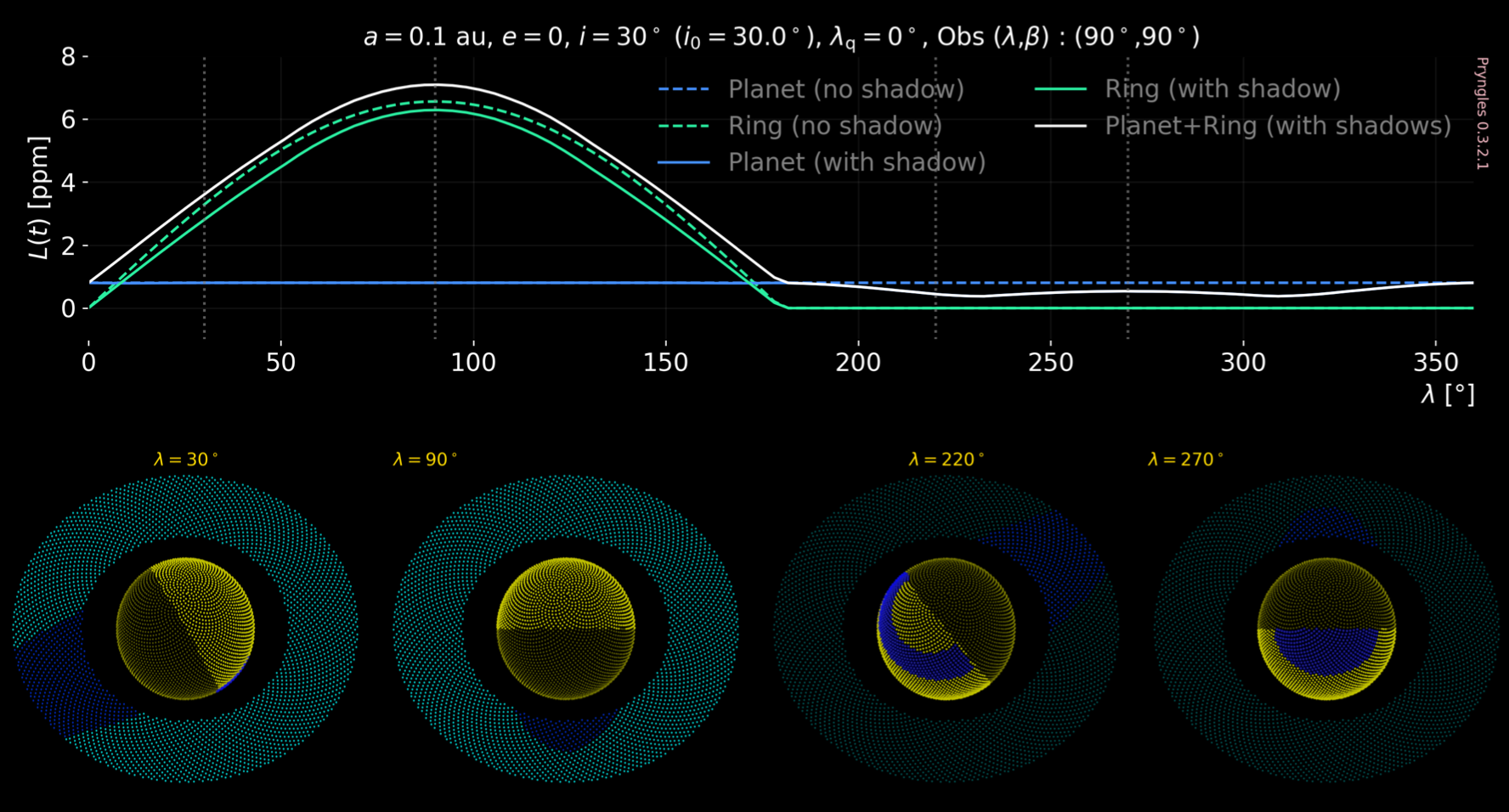
This is an example of what can be done with Pryngles:
API Documentation
You can explore detailed descriptions of all classes, functions, and modules at:
👉 https://pryngles.readthedocs.io
This resource will be updated as the package evolves. We welcome your feedback and suggestions!
Download and Install
From PyPI:
Pryngles is available in PyPI, https://pypi.org/project/pryngles/.
To install it, just execute:
pip install -Uq pryngles
From soruces:
If you prefer, you may download from the sources or directly from our GitHub repository.
$ git clone https://github.com/seap-udea/pryngles
To install the package from the sources use the following command in your terminal:
$ cd pryngles
$ pip install .
In case you want to contribute to our package, please use an editable installing
$ cd pryngles
$ pip install -e .
In GoogleColab:
If you are used to GoogleColab environment, you may also install pryngles by executing:
!pip install -Uq pryngles
Tutorials
We have prepared several Jupyter tutorials to guide you in the usage
of the package. The tutorials evolve as the package is being optimized.
-
Quickstart [Download, Google Colab]. In this tutorial you will learn the very basics about the package.
-
Developers [Download, Google Colab]. In this tutorial you will find a detailed description and exemplification of almost every part of the package. It is especially intended for developers, however it may also be very useful for finding code snippets useful for science applications. As expected, it is under construction as the package is being developed.
Examples
Working with Pryngles we have created several Jupyter notebooks to
illustrate many of its capabilities. In the examples below you will
find the package at work to do actual science:
- Full-science exploration [Download, Google Colab]. In this example we include the code we used to generate the plots of the release paper arXiv:2207.08636 as a complete example of how the package can be used in a research context.
Development with AI
Pryngles is possibly one of the last photometric/polarimetric forward-modeling packages that started out before the arrival of large language models (LLMs). Today, these models can substantially accelerate tasks that used to take months or years: exploring and understanding legacy code, test-guided refactoring, generating technical documentation, and systematically reviewing numerical edge cases.
Starting with version 1.0.0, we have begun to introduce (gradually and carefully) LLM-assisted workflows to review and improve aspects of the package, in particular:
- reviewing and updating examples and tutorials;
- detecting incompatibilities introduced by upstream scientific libraries (e.g.,
pandas,scipy); - improving documentation and reproducible usage guides.
The goal is not to “automate science”, but to reduce iteration time so the team can focus on what matters most: physical validation, numerical robustness, and usability.
Contributions
This project started as an effort to extend and operationalize the ideas presented in Sucerquia et al. (2020). It was initially developed by Jorge I. Zuluaga. Later, Mario Sucerquia and Jaime A. Alvarado-Montes joined the development, especially as beta testers and developers who used the package as a research tool to produce the scientific results.
Later, Allard K. Veenstra joined the team and developed the polarization capabilities in the RingedPlanet interface, contributing to the consolidation of the polarimetric model. The most recent developer to join the team was Sebastian Numpaque, who implemented much of the recent paper’s innovations in the System interface and led the technical documentation.
In addition to the above, we acknowledge direct or indirect contributions from:
- Daphne M. Stam: co-author of the polarimetric paper; her long-standing work in photometry/polarimetry and references to historical codes/tools (including Fortran implementations for computing and validating scattering/polarization coefficients and phase behavior) were key to validating and benchmarking our models.
What's new
For a detailed list of the newest features introduced in the latest releases please check What's new.
Quickstart
Please import the package and some useful utilities:
import pryngles as pr
from pryngles import Consts
NOTE: If you are working in
GoogleColabbefore producing any plot please load the matplotlib backend:
%matplotlib inline
Pryngles currently exposes two interfaces. The legacy interface is called RingedPlanet; it was used in the earliest versions of the package and in part of the published scientific work. We keep it for a limited transition period so older research code and notebooks remain reproducible. Examples based on this interface are available in tutorials/Quickstart-RingedPlanet.ipynb and in the legacy-oriented examples below. The modern interface is System, which is the most flexible interface in the package because it supports more complex configurations such as planets with rings, moons, multiple stars, and thermal-emission workflows.
System (official) interface
The recommended quickstart for new work is the System interface. A complete executable version of the workflow is available in tutorials/Quickstart-System.ipynb.
Create a star, a planet, and a ring:
import pryngles as pr
import numpy as np
import spiceypy as spy

system = pr.System()

star = system.add(
  kind='Star',
  radius=pr.Consts.rsun / system.ul,
  limb_coeffs=[0.65],
)

planet = system.add(
  kind='Planet',
  parent=star,
  a=0.2,
  e=0.0,
  radius=pr.Consts.rsaturn / system.ul,
)

ring = system.add(
  kind='Ring',
  parent=planet,
  fi=1.5,
  fe=2.5,
  i=30 * pr.Consts.deg,
)
Set the observer geometry, initialize the dynamics, discretize the surfaces, and visualize the system:
inc = 90.0
omega = 0.0
system.n_obs = spy.eul2m(np.deg2rad(omega), np.deg2rad(inc), 0, 3, 1, 3)[0]

system.initialize_simulation()
system.spangle_system()
system.integrate_perspective(0)
system.sg.plot2d()
system.sg.fig2d.savefig('gallery/simple_system_view.png', dpi=300)
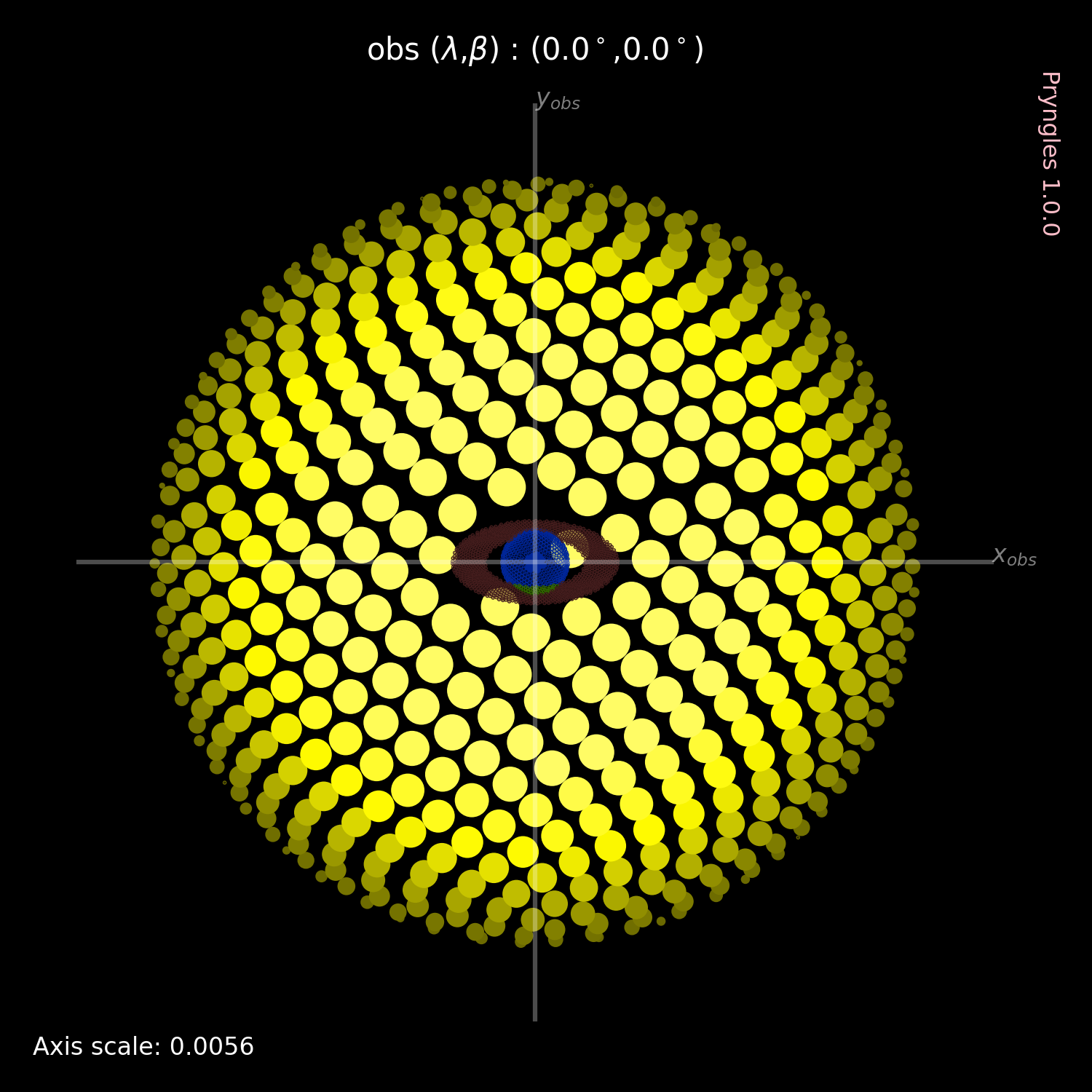
This produces the following system view:
Compute the reflected/scattered flux and polarization over one orbital cycle:
n_times = 181
period_days = 365.25 * (planet.a ** 1.5)
times_days = np.linspace(0.0, period_days, n_times)
times_system = times_days * pr.Consts.day / system.ut

system.compute_lightcurve(
  times=times_system,
  effects=['polarization'],
)

scattering_df = system.lightcurve['scattering']
polarization_df = system.lightcurve['polarization']
The important difference with respect to RingedPlanet is that System stores the results in pandas objects. This makes it easy to extract the contribution from each body and then combine them explicitly:
planet_flux = scattering_df['Planet']
ring_flux = scattering_df['Ring']
total_flux = scattering_df.sum(axis=1)

planet_flux_ppm = pr.Consts.ppm * planet_flux
ring_flux_ppm = pr.Consts.ppm * ring_flux
total_flux_ppm = pr.Consts.ppm * total_flux

planet_pol = polarization_df['Planet']
ring_pol = polarization_df['Ring']
total_pol = polarization_df.sum(axis=1)
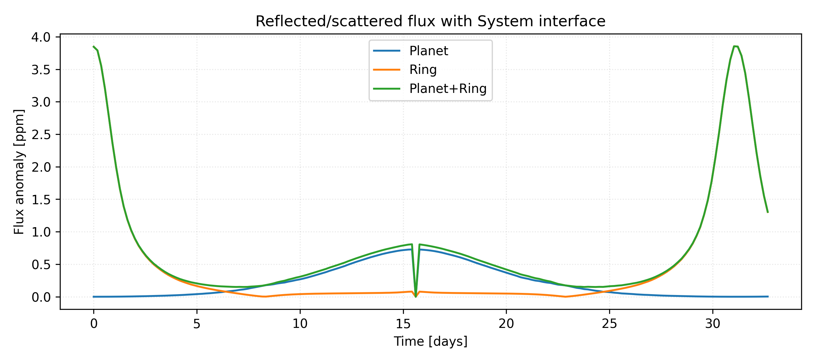
The resulting reflected/scattered flux can then be plotted exactly as in the legacy quickstart, but now using the System outputs:
And the polarization workflow gives access to both the flux components and the polarization degree for Planet, Ring, and the combined system:
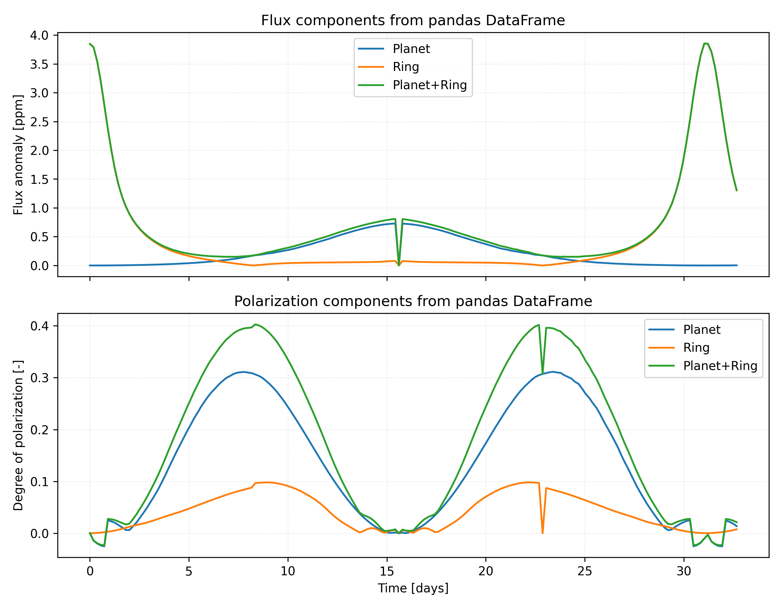
For the full step-by-step notebook, including the pandas extraction logic and plotting code, see tutorials/Quickstart-System.ipynb.
RingedPlanet (legacy) interface
Any calculation in Pryngles starts by creating a planetary system:
sys = pr.System()

S = sys.add(kind = "Star", radius = Consts.rsun/sys.ul, limb_coeffs = [0.65])
P = sys.add(kind = "Planet",parent = S, a = 0.2, e = 0.0, radius = Consts.rsaturn/sys.ul)
R = sys.add(kind = "Ring", parent = P, fi = 1.5, fe = 2.5, i = 30*Consts.deg)
In the example before the planet has a ring extending from 1.5 to 2.5 planetary radius which is inclined 30 degrees with respect to the orbital plane. It has an orbit with semimajor axis of 0.2 and eccentricity 0.0.
NOTE: The following section implements our previous
RingedPlanetinterface, which is limited to modeling simple systems. If you would like to use our new, still-in-development interfaceSystem, please refer to our Tutorials section.
Once the system is set we can ensamble a simulation, ie. creating an object able to produce a light-curve.
RP = sys.ensamble_system()
To see how the surface of the planet and the rings looks like run:
RP.plotRingedPlanet()
You may change the position of the star in the orbit and see how the appearance of the planet changes:
RP.changeStellarPosition(45*Consts.deg)
RP.plotRingedPlanet()
Below is the sequence of commands to produce your first light curve:
import numpy as np

RP.changeObserver([90*Consts.deg, 30*Consts.deg])
lambs = np.linspace(0.0*Consts.deg, 360*Consts.deg, 100)
Rps = []
Rrs = []
ts = []

for lamb in lambs:
    RP.changeStellarPosition(lamb)
    ts += [RP.t*sys.ut/Consts.day]
    RP.updateOpticalFactors()
    RP.updateDiffuseReflection()
    Rps += [RP.Rip.sum()]
    Rrs += [RP.Rir.sum()]

ts = np.array(ts)
Rps = np.array(Rps)
Rrs = np.array(Rrs)

#Plot
import matplotlib.pyplot as plt
fig = plt.figure()
ax = fig.gca()
ax.plot(ts, Consts.ppm*Rps, label = "Planet")
ax.plot(ts, Consts.ppm*Rrs, label = "Ring")
ax.plot(ts, Consts.ppm*(Rps + Rrs), label = "Planet+Ring")

ax.set_xlabel("Time [days]")
ax.set_ylabel("Flux anomaly [ppm]")
ax.legend();
And voilà!
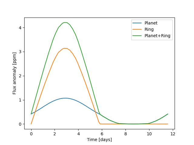
Let's have some Pryngles.
Realistic Scattering and Polarization
Starting in version 0.9.x, Pryngles is able to compute fluxes using a more realistic model for scattering that includes polarization. The new features are not yet flexible enough but they can be used to create more realistic light curves.
These new features are based on the science and Fortran code developed
by Prof. Daphne Stam and collaborators, and adapted to Pryngles
environment by Allard Veenstra (Fortran and Python wrapping) and Jorge
I. Zuluaga (translation to C and ctypes). For the science behind the
scattering and polarization code see:
Rossi, L., Berzosa-Molina, J., & Stam, D. M. (2018). PyMieDAP: a Python–Fortran tool for computing fluxes and polarization signals of (exo) planets. Astronomy & Astrophysics, 616, A147. arXiv:1804.08357
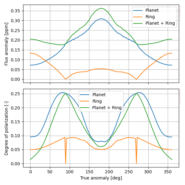
Below is a simple example of how to compute the light curve of a ringed planet whose atmosphere and ring scatters reallistically the light of the star. The code compute the components of the Stokes vector and the degree of polarization of the diffusely reflected light on the system.
As shown in the example before, we first need to create the system:
nspangles = 1000

sys = pr.System()

S = sys.add(kind = "Star", radius = Consts.rsun/sys.ul, limb_coeffs = [0.65])
P = sys.add(kind = "Planet", primary = S, a = 3, e = 0.0,
          radius = Consts.rsaturn/sys.ul, nspangles = nspangles)
R = sys.add(kind = "Ring", primary = P, fi = 1.5, fe = 2.25,
          i = 30*Consts.deg, roll = 90*Consts.deg, nspangles = nspangles)

RP = sys.ensamble_system()
Then generate the light curve:
import numpy as np
from tqdm import tqdm

RP.changeObserver([-90*Consts.deg, 60*Consts.deg])
lambs = np.linspace(90*Consts.deg, 450*Consts.deg, 181)

ts = []
Rps = []
Rrs = []
Pp  =  []
Pr  =  []
Ptot = []
for lamb in tqdm(lambs):
    RP.changeStellarPosition(lamb)
    ts += [RP.t*RP.CU.UT]
    RP.updateOpticalFactors()
    RP.updateReflection()
    Rps += [RP.Rip.sum()]
    Rrs += [RP.Rir.sum()]
    Pp +=  [RP.Ptotp]
    Pr +=  [RP.Ptotr]
    Ptot += [RP.Ptot]

ts = np.array(ts)
Rps = np.array(Rps)
Rrs = np.array(Rrs)
Pp = np.array(Pp)
Pr = np.array(Pr)
Ptot = np.array(Ptot)
And plot it:
#Plot
fig, axs = plt.subplots(2, 1, figsize = (6, 6), sharex = True)

ax = axs[0]
ax.plot(lambs*180/np.pi-90, Rps, label = "Planet")
ax.plot(lambs*180/np.pi-90, Rrs, label = "Ring")
ax.plot(lambs*180/np.pi-90, Rps+Rrs, label = "Planet + Ring")
ax.set_ylabel("Flux anomaly [ppm]")
ax.legend()
ax.grid()
pr.Plot.pryngles_mark(ax)

ax = axs[1]
ax.plot(lambs*180/np.pi-90, Pp, label = "Planet")
ax.plot(lambs*180/np.pi-90, Pr, label = "Ring")
ax.plot(lambs*180/np.pi-90, Ptot, label = "Planet + Ring")
ax.set_ylabel("Degree of polarization [-]")
ax.legend()
ax.grid()
pr.Plot.pryngles_mark(ax)

ax = axs[1]
ax.set_xlabel("True anomaly [deg]")
fig.tight_layout()
The resulting polarization and light-curve will be:
This package has been designed and written originally by Jorge I. Zuluaga, Allard Veenstra, Sebastian Numpaque, Mario Sucerquia and Jaime A. Alvarado-Montes (C) 2022-Present.
Project details
Release history Release notifications | RSS feed


Download files
Download the file for your platform. If you're not sure which to choose, learn more about installing packages.
Source Distribution
Built Distribution
Filter files by name, interpreter, ABI, and platform.
If you're not sure about the file name format, learn more about wheel file names.
Copy a direct link to the current filters
File details
Details for the file pryngles-1.0.2.tar.gz.
File metadata
- Download URL: pryngles-1.0.2.tar.gz
- Upload date:
- Size: 21.0 MB
- Tags: Source
- Uploaded using Trusted Publishing? No
- Uploaded via: twine/6.2.0 CPython/3.13.3
File hashes
| Algorithm | Hash digest | |
|---|---|---|
| SHA256 |
a3e03f2c863ba4f5400c11ac8772ac6fcedf3ac491996aa37acb30f51a4d8421
|
|
| MD5 |
b10c8a376455c6f19e848a566cafa5d2
|
|
| BLAKE2b-256 |
44b717be9c47553e298de0ba5beaa876fc3721e1133a502696a9cd2d899eb8fe
|
File details
Details for the file pryngles-1.0.2-cp313-cp313-macosx_14_0_arm64.whl.
File metadata
- Download URL: pryngles-1.0.2-cp313-cp313-macosx_14_0_arm64.whl
- Upload date:
- Size: 21.7 MB
- Tags: CPython 3.13, macOS 14.0+ ARM64
- Uploaded using Trusted Publishing? No
- Uploaded via: twine/6.2.0 CPython/3.13.3
File hashes
| Algorithm | Hash digest | |
|---|---|---|
| SHA256 |
6a57ff3411d899eff0e870de897483c404957b8fd39f67662dcf5f91e6af8d13
|
|
| MD5 |
5f8e187b0f50ec76cb8404839569aa21
|
|
| BLAKE2b-256 |
4732c5411de864332fb917bea5e56476dc5f3cc99b930c25451f1b13491d2a95
|






