
pyEllipse
A Python library for computing Hotelling's T² statistics and generating confidence ellipse/ellipsoid coordinates for multivariate data analysis and visualization.










Overview
pyEllipse provides three functions for multivariate data:
hotelling_parameters- Hotelling's T² statistic of each observation, its cutoffs, and the semi-axes and rotation of Hotelling's ellipsehotelling_coordinates- Points of Hotelling's ellipse (2D) or ellipsoid (3D) of PCA, PLS or other component scoresconfidence_ellipse- Confidence ellipses and ellipsoids of raw data, optionally by group and with robust estimates
The documentation gives the theory behind each function, worked examples, and the API reference.
Installation
pip install pyEllipse
Usage Examples
The examples use the wine data of scikit-learn (178 samples, 13 measurements, 3 cultivars). Their figures are ready for publication: sized for journal columns, they keep their size when saved, embed their fonts, and remain readable in grayscale and with colour-vision deficiencies. They use the following matplotlib settings:
Figure style
import matplotlib.pyplot as plt
from cycler import cycler

# Figure widths of most journals, in inches: single, 1.5 and double column
MM = 1 / 25.4
SINGLE, ONE_HALF, DOUBLE = 89 * MM, 140 * MM, 183 * MM

# Colour-blind-safe colours, used in this order; each figure also varies line style
# or marker shape, so it can be printed in grayscale
BLUE, ORANGE, AQUA, GREY = "#2a78d6", "#eb6834", "#1baf7a", "#808080"

plt.rcParams.update({
    # Text and mathematics in the same sans-serif font, at the printed size
    "font.family": "sans-serif",
    "font.sans-serif": ["Arial", "Helvetica", "Liberation Sans", "DejaVu Sans"],
    "font.size": 9,
    "axes.labelsize": 9,
    "xtick.labelsize": 8,
    "ytick.labelsize": 8,
    "legend.fontsize": 8,
    "mathtext.fontset": "custom",
    "mathtext.rm": "sans",
    "mathtext.it": "sans:italic",
    "mathtext.bf": "sans:bold",
    "mathtext.sf": "sans",
    "mathtext.cal": "sans:italic",
    # Thin black axes, outward ticks, no grid
    "axes.edgecolor": "black",
    "axes.linewidth": 0.6,
    "axes.spines.top": False,
    "axes.spines.right": False,
    "axes.prop_cycle": cycler(color=[BLUE, ORANGE, AQUA]),
    "xtick.major.width": 0.6,
    "ytick.major.width": 0.6,
    "xtick.major.size": 3,
    "ytick.major.size": 3,
    "xtick.direction": "out",
    "ytick.direction": "out",
    "lines.linewidth": 1.2,
    "legend.frameon": False,
    # Saved figures keep the exact size set with figsize
    "figure.constrained_layout.use": True,
    # Vector output with embedded TrueType fonts; 600 dpi for raster formats
    "pdf.fonttype": 42,
    "ps.fonttype": 42,
    "svg.fonttype": "none",
    "savefig.dpi": 600,
})
Save a figure in the format your journal requires, e.g. fig.savefig("figure.pdf") or fig.savefig("figure.tiff", dpi=600).
Example 1: Hotelling's T² statistic and ellipses from PCA scores
import numpy as np
import pandas as pd
from matplotlib.colors import LinearSegmentedColormap
from matplotlib.lines import Line2D
from sklearn.datasets import load_wine
from sklearn.decomposition import PCA
from sklearn.preprocessing import StandardScaler

from pyEllipse import confidence_ellipse, hotelling_coordinates, hotelling_parameters

wine = load_wine()
X = StandardScaler().fit_transform(wine.data)
pca = PCA().fit(X)
scores = pca.transform(X)
explained = pca.explained_variance_ratio_

# T² on PC1 and PC2, with the exact limits for the samples the model was fitted on
res = hotelling_parameters(scores, pcx=1, pcy=2, method="beta")
t2 = res["Tsquared"]["value"]
ellipse_95 = hotelling_coordinates(scores, pcx=1, pcy=2, conf_limit=0.95, method="beta")
ellipse_99 = hotelling_coordinates(scores, pcx=1, pcy=2, conf_limit=0.99, method="beta")
# Sequential colour map, light to dark, for the magnitude of T²
t2_cmap = LinearSegmentedColormap.from_list(
    "t2", ["#86b6ef", "#5598e7", "#2a78d6", "#1c5cab", "#104281"]
)

fig, ax = plt.subplots(figsize=(ONE_HALF, 94 * MM))
points = ax.scatter(scores[:, 0], scores[:, 1], c=t2, cmap=t2_cmap, s=12,
                    edgecolor="white", linewidth=0.3, zorder=3)
for ellipse, label, style in [(ellipse_95, "95%", "--"), (ellipse_99, "99%", "-")]:
    ax.plot(ellipse["x"], ellipse["y"], color="black", lw=0.9, ls=style)
    top = ellipse["y"].idxmax()
    ax.annotate(label, (ellipse["x"][top], ellipse["y"][top]), xytext=(0, 2),
                textcoords="offset points", ha="center", va="bottom")
fig.colorbar(points, ax=ax, label=r"$T^2$ (PC1 and PC2)", shrink=0.75, aspect=25)
ax.set_aspect("equal", adjustable="datalim")
ax.set_xlabel(f"PC1 ({explained[0]:.1%})")
ax.set_ylabel(f"PC2 ({explained[1]:.1%})")
plt.show()
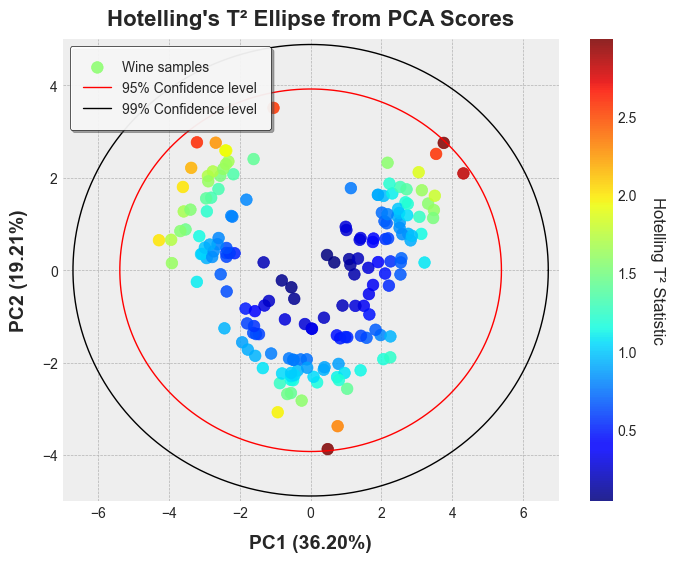
The Tsquared values are on the same scale as the cutoffs, so a sample lies outside the ellipse exactly when its T² exceeds the corresponding cutoff. To flag outliers on more components, set k or threshold; conf_limit sets the confidence levels:
res_80 = hotelling_parameters(scores, threshold=0.8, method="beta", conf_limit=(0.95, 0.99))
t2_80 = res_80["Tsquared"]["value"]
outliers = np.flatnonzero(t2_80 > res_80["cutoff_99pct"])
method="beta" gives the exact limits for the samples the model was fitted on; the default method="f" is more conservative for small samples. When the components are correlated, e.g. new samples projected onto a model, the ellipse is rotated; its rotation is returned in res["Ellipse"]["angle"] (0 for PCA scores).
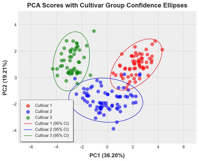
Example 2: Confidence ellipses by group
df = pd.DataFrame(scores[:, :3], columns=["PC1", "PC2", "PC3"])
df["Cultivar"] = [f"Cultivar {target + 1}" for target in wine.target]

ellipses = confidence_ellipse(df, x="PC1", y="PC2", group_by="Cultivar",
                              conf_level=0.95, robust=True, distribution="hotelling")

# Colour, marker and line style of each cultivar
styles = {"Cultivar 1": (BLUE, "o", "-"), "Cultivar 2": (ORANGE, "^", "--"),
          "Cultivar 3": (AQUA, "s", "-.")}

fig, ax = plt.subplots(figsize=(ONE_HALF, 94 * MM))
for cultivar, (color, marker, style) in styles.items():
    group = df[df["Cultivar"] == cultivar]
    ellipse = ellipses[ellipses["Cultivar"] == cultivar]
    ax.scatter(group["PC1"], group["PC2"], s=12, marker=marker, color=color,
               edgecolor="white", linewidth=0.3, zorder=3)
    ax.plot(ellipse["x"], ellipse["y"], color=color, lw=1.2, ls=style)
handles = [Line2D([], [], color=color, marker=marker, ls=style, lw=1.2, markersize=4,
                  markeredgecolor="white", markeredgewidth=0.3, label=cultivar)
           for cultivar, (color, marker, style) in styles.items()]
fig.legend(handles=handles, loc="outside upper center", ncols=3)
ax.set_aspect("equal", adjustable="datalim")
ax.set_xlabel(f"PC1 ({explained[0]:.1%})")
ax.set_ylabel(f"PC2 ({explained[1]:.1%})")
plt.show()
Example 3: Confidence ellipsoids by group
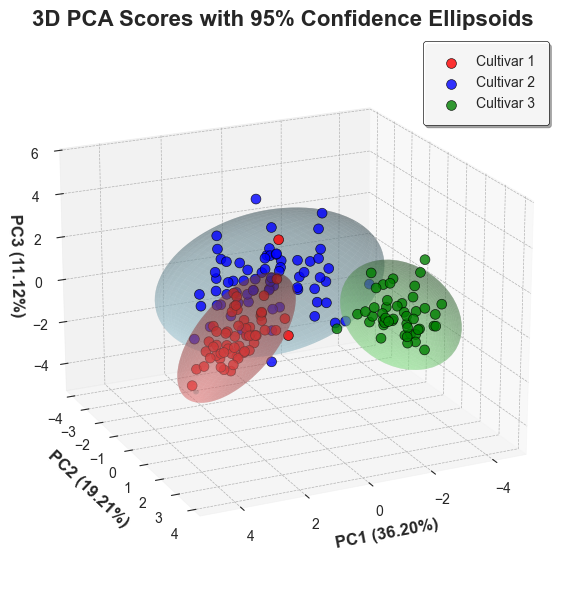
ellipsoids = confidence_ellipse(df, x="PC1", y="PC2", z="PC3", group_by="Cultivar",
                                conf_level=0.95, robust=True, distribution="hotelling")

fig = plt.figure(figsize=(ONE_HALF, 110 * MM))
ax = fig.add_subplot(projection="3d")
for cultivar, (color, marker, _) in styles.items():
    group = df[df["Cultivar"] == cultivar]
    ellipsoid = ellipsoids[ellipsoids["Cultivar"] == cultivar]
    side = int(np.sqrt(len(ellipsoid)))  # the points form a side x side grid
    x, y, z = (ellipsoid[c].to_numpy().reshape(side, side) for c in ["x", "y", "z"])
    ax.plot_wireframe(x, y, z, rstride=5, cstride=5, color=color, lw=0.4)
    ax.scatter(group["PC1"], group["PC2"], group["PC3"], s=8, marker=marker,
               color=color, depthshade=False, label=cultivar)
for axis in (ax.xaxis, ax.yaxis, ax.zaxis):
    axis.pane.fill = False
ax.grid(False)
ax.set_xlabel(f"PC1 ({explained[0]:.1%})")
ax.set_ylabel(f"PC2 ({explained[1]:.1%})")
ax.set_zlabel(f"PC3 ({explained[2]:.1%})")
ax.legend(loc="upper left")
plt.show()
Key Differences Between Functions
| Feature | hotelling_parameters |
hotelling_coordinates |
confidence_ellipse |
|---|---|---|---|
| Input | Component scores | Component scores | Raw data |
| Purpose | T² statistics | Plot coordinates | Plot coordinates |
| Grouping | -- | -- | Yes |
| Robust | -- | -- | Yes |
| 2D/3D | 2D only for ellipse params | Both | Both |
| Distribution | Hotelling only | Hotelling only | Normal or Hotelling |
| Use Case | Outlier detection, QC | Visualizing PCA | Exploratory data analysis |
When to Use Each Function
Use hotelling_parameters when:
- You need T² statistics for outlier detection
- You want confidence cutoff values
- You're performing quality control or process monitoring
- You need ellipse parameters (semi-axes lengths)
Use hotelling_coordinates when:
- You have PCA/PLS component scores
- You want to visualize confidence regions on score plots
- You need precise control over which components to plot
- You're creating publication-quality figures from multivariate models
Use confidence_ellipse when:
- You're working with raw data (not scores)
- You need to compare multiple groups
- You want robust estimation for outlier-resistant analysis
- You need flexibility in distribution choice (normal vs Hotelling)
Citation
If you use pyEllipse in your research, please cite it:
@software{goueguel_pyellipse,
  author  = {Goueguel, Christian L.},
  title   = {{pyEllipse: Statistical confidence ellipses and Hotelling's T-squared ellipses}},
  year    = {2026},
  version = {0.2.1},
  url     = {https://github.com/ChristianGoueguel/pyEllipse},
  license = {MIT}
}
A machine-readable CITATION.cff is also included, so GitHub's "Cite this repository" button stays in sync.
References
- Hotelling, H. (1931). The generalization of Student's ratio. Annals of Mathematical Statistics, 2(3), 360-378.
- Brereton, R. G. (2016). Hotelling's T-squared distribution, its relationship to the F distribution and its use in multivariate space. Journal of Chemometrics, 30(1), 18-21.
- Tracy, N. D., Young, J. C., & Mason, R. L. (1992). Multivariate control charts for individual observations. Journal of Quality Technology, 24(2), 88-95.
- Rousseeuw, P. J., & Van Driessen, K. (1999). A fast algorithm for the minimum covariance determinant estimator. Technometrics, 41(3), 212-223.
- Jackson, J. E. (1991). A User's Guide to Principal Components. Wiley.
1 maintainer

Metadata
1 maintainer
Release files for pyEllipse 0.2.1
For a detailed explanation of source distributions (sdists) and built distributions (wheels), please see the package formats documentation.
Source distribution (sdist)
| File | Size | Uploaded | |
|---|---|---|---|
| pyellipse-0.2.1.tar.gz | 21.2 kB | Details |
Built distribution (wheel)
| File | Interpreter | ABI | Platform | Reset |
|---|---|---|---|---|
| pyellipse-0.2.1-py3-none-any.whl | Python 3 | none | any | Details |
Total release size: 41.6 kB
Release files / pyellipse-0.2.1.tar.gz
| Download URL | pyellipse-0.2.1.tar.gz |
|---|---|
| Size | 21.2 kB |
| Tags | Source |
|
SHA-256 checksum How to use checksums |
86d478f691c0cb5e2227e6bae60ff304279d1e363607d735733bc0360405ab59
|
|
BLAKE2b-256 checksum How to use checksums |
07ac4e0ab09fc489217a6cc2b5b647650f88d5d3f525b3b6dcbc42c93e393313
|
| Upload date | |
|
Uploaded using Trusted Publishing? What is trusted publishing? |
No |
| Uploaded via |
poetry/2.2.0 CPython/3.13.7 Darwin/25.6.0
|
Release files / pyellipse-0.2.1-py3-none-any.whl
| Download URL | pyellipse-0.2.1-py3-none-any.whl |
|---|---|
| Size | 20.5 kB |
| Tags | Python 3 |
|
SHA-256 checksum How to use checksums |
3301e4cbd7ffceda4fd293f7c9b0bb8483d24292e938bcd36aae88e3f460eb5f
|
|
BLAKE2b-256 checksum How to use checksums |
6f7c688d0ab0eaeda686417475c41b7b7cc2d7425e774d31d902256ffb851cda
|
| Upload date | |
|
Uploaded using Trusted Publishing? What is trusted publishing? |
No |
| Uploaded via |
poetry/2.2.0 CPython/3.13.7 Darwin/25.6.0
|














