A stochastic model for the modeling of DNA replication and cell-cycle dynamics.

Project description
RepliSage
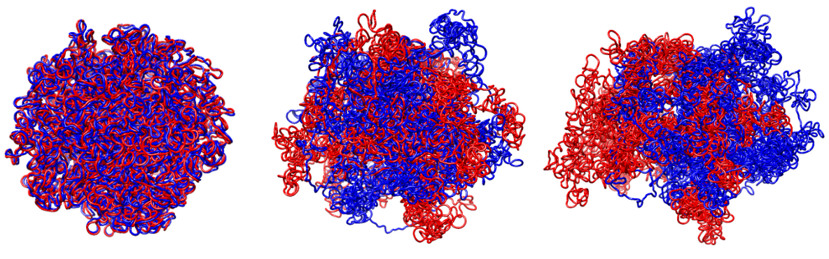
A simulation software for modeling the motion of cohesin during the replication process. This tool explores the interaction between cohesin, or more generally loop extrusion factors (LEFs), with replication forks and chromatin compartmentalization. It employs a sophisticated force-field that integrates MCMC Metropolis and molecular dynamics methodologies. The output is a 3D chromatin trajectory, providing a dynamic visualization of DNA replication and the formation of two identical copies.
Simulation pipeline
RepliSage is composed by three distinct parts:
Replication simulation (Replikator.py)
This is a simplistic Monte Carlo simulation, where we import single cell replication timing data to model replication. The average replication timing curves can show us the percentage of cells that have been replicated, and from them we estimate the initiation rate $I(x,t)$ which represents the probability fires at time $t$ in loci $x$. Then we employ the Monte Carlo simulation where in each step an origin fires with a probability derived from the initiation rate. When an origin fires, the replication fork start propagating bi-directionally with velocity $v$. The vlocity's mean and standard deviation is derived by calculating the slopes of consecutive optima of the averaged replication timing curve. Replikator outputs the trajectories of the replication forks.
Stochastic simulation that models the interplay of loop extrusion with other factors
In this part we import the previously produced trajectories of replication forks and we model them as moving barriers for the loop extrusion factors. In this way this simulation is composed by three distinct parts:
Loop Extrusion
We use the energy landscape of LoopSage for that. We assume that there are two basic players: LEFs which follow a random difussive motion in 1D and CTCF whose locations are dervied from ChIA-PET data, which are filtered where is a CTCF motif in their sequence. Therefore, assuming that we have $N_{\text{lef}}$ LEFs with two degrees of freedom $(m_i,n_i)$ and epigenetic color states $s_i$ for each monomer, we can write down the following formula,
$$E_{\text{le}} = c_{\text{fold}}\sum_{i=1}^{N_{\text{coh}}}\log(n_i-m_i)+c_{\text{cross}}\sum_{i,j}K(m_i,n_i;m_j,n_j)+c_{\text{bind}}\sum_{i=1}^{N_{\text{coh}}}\left(L(m_i)+R(n_i)\right).$$
In this equation the first term models the folding of chromatin (how fast a loop extrudes, the higher $f$ the more tendency to extrude), the second term is a penalty for cohesin crossing, and the last one minimizes the energy when a LEF encounters a CTCF.
Compartmentalization
It is modelled by using a five stats ($s_i\in[-2,-1,0,1,2]$) Potts model
$$E_{\text{potts}} = C_{p,1} \sum_{k} \left(\dfrac{h_k + h_{t_{r} k}}{2} \right) s_k +C_{p,2}\sum_{i>j} J_{ij}| s_i - s_j |.$$
The second term includes the interaction matrix $J_{ij}$, which is 1 when there is a LEF connecting $i$ with $j$ and 0 if not. The other term represents an epigeetic field. There is an averaged term $h_k$, which represents the averaged replication timing, and a time dependent term $h_{t_{r} k}$ which represents the spread of the epigenetic state due to a single replication fork.
Replication
This term models the interaction between the LEFs and replication forks, $$E_{\text{rep}}=C_{\text{rep}}\sum_{i=1}^{N_{lef}} \mathcal{R}(m_i,n_i ;f_{\text{rep}})$$ and in general penalizes inapropriate configurations between LEFs and replication forks (read the paper).
Therefore, the stochastic simulation integrates the sum of these energies $E = E_{le}+E_{rep}+E_{potts}$ and uses MCMC Metropolis method.
Molecular Dynamics
This parts takes as input the states produced by the stochastic simulation and outputs 3D structures by using a potential in OpenMM. The molecular modeling approach assumes two molecular chains, each consisting of $N_{\text{beads}}$ monomers, where $N_{\text{beads}}$ reflects the granularity of the stochastic simulation. The total potential governing the system is expressed as: $$U = U_{\text{bk}} + U_{\text{le}}(t) + U_{\text{rep}}(t) + U_{\text{block}}(t)$$, where each term corresponds to a specific contribution. The backbone potential ($U_{\text{bk}}$) includes strong covalent bonds between consecutive beads, angular forces, and excluded volume effects to maintain chain integrity. The loop-formation potential ($U_{\text{le}}$) is a time-dependent term introducing harmonic bonds to model loop formation. These bonds are weaker than the backbone interactions and act between dynamically changing pairs of beads, $m_i(t)$ and $n_i(t)$. The last term models compartmentalization with block-copolymer potential.
For more details of the implementation, we suggest to our users to read the method paper of RepliSage.
Installation
It is needed to have at least python 3.10 and run,
pip install -r requirements.txt
Or more easily (do not forget to install it with python 3.10 or higher),
pip install pyRepliSage
How to use?
The usage is very simple. To run this model you need to specify the parameters and the input data. Then RepliSage can do everything for you.
Note that to run replisage it is needed to have GM12878_single_cell_data_hg37.mat data, for single-cell replication timing. These data are not produced by our laboratory, but they are alredy published in the paper of D. S. Massey et al. Please do not forget to cite them. We have uploaded the input data used in the paper here: https://drive.google.com/drive/folders/1PLA147eiHenOw_VojznnlC_ZywhLzGWx?usp=sharing.
Python API
from RepliSage.stochastic_model import *

# Set parameters
N_beads, N_lef, N_lef2 = 1000, 100, 20
N_steps, MC_step, burnin, T, T_min, t_rep, rep_duration = int(8e4), int(4e2), int(1e3), 1.6, 1.0, int(1e4), int(2e4)

f, f2, b, kappa= 1.0, 5.0, 1.0, 1.0
c_state_field, c_state_interact, c_rep = 2.0, 1.0, 1.0
mode, rw, random_spins, rep_fork_organizers = 'Metropolis', True, True, True
Tstd_factor, speed_scale, init_rate_scale, p_rew = 0.1, 20, 1.0, 0.5
save_MDT, save_plots = True, True

# Define data and coordinates
region, chrom =  [80835000, 98674700], 'chr14'

# Data
bedpe_file = '/home/skorsak/Data/method_paper_data/ENCSR184YZV_CTCF_ChIAPET/LHG0052H_loops_cleaned_th10_2.bedpe'
rept_path = '/home/skorsak/Data/Replication/sc_timing/GM12878_single_cell_data_hg37.mat'
out_path = '/home/skorsak/Data/Simulations/RepliSage_whole_chromosome_14'

# Run simulation
sim = StochasticSimulation(N_beads, chrom, region, bedpe_file, out_path, N_lef, N_lef2, rept_path, t_rep, rep_duration, Tstd_factor, speed_scale, init_rate_scale)
sim.run_stochastic_simulation(N_steps, MC_step, burnin, T, T_min, f, f2, b, kappa, c_rep, c_state_field, c_state_interact, mode, rw, p_rew, rep_fork_organizers, save_MDT)
if show_plots: sim.show_plots()
sim.run_openmm('OpenCL',mode='MD')
if show_plots: sim.compute_structure_metrics()

# Save Parameters
if save_MDT:
    params = {k: v for k, v in locals().items() if k not in ['args','sim']}
    save_parameters(out_path+'/other/params.txt',**params)
Bash command
An even easier way that you can avoid all python coding is by running the command,
replisage -c config.ini
The configuration file has the usual form,
[Main]

; Input Data and Information
BEDPE_PATH = /home/blackpianocat/Data/method_paper_data/ENCSR184YZV_CTCF_ChIAPET/LHG0052H_loops_cleaned_th10_2.bedpe
REPT_PATH = /home/blackpianocat/Data/Replication/sc_timing/GM12878_single_cell_data_hg37.mat
REGION_START = 80835000
REGION_END = 98674700
CHROM = chr14
PLATFORM = CUDA
OUT_PATH = /home/blackpianocat/Data/Simulations/RepliSage_test

; Simulation Parameters
N_BEADS = 2000
N_LEF = 200
BURNIN = 1000
T_INIT = 1.8
T_FINAL = 1.0
METHOD = Metropolis
LEF_RW = True
RANDOM_INIT_SPINS = True

; Molecular Dynamics
INITIAL_STRUCTURE_TYPE = rw
SIMULATION_TYPE = MD
TOLERANCE = 1.0
EV_P=0.01
You can define these parameters based on the table of simulation parameters.
Parameter table
| Parameter Name | Type | Default Value |
|---|---|---|
| PLATFORM | str | CPU |
| DEVICE | str | '' |
| N_BEADS | int | '' |
| BEDPE_PATH | str | '' |
| REPT_PATH | str | '' |
| OUT_PATH | str | ../results |
| REGION_START | int | '' |
| REGION_END | int | '' |
| CHROM | str | '' |
| REP_T_STD_FACTOR | float | 0.1 |
| REP_SPEED_SCALE | float | 20 |
| REP_INIT_RATE_SCALE | float | 1.0 |
| LEF_RW | bool | True |
| RANDOM_INIT_SPINS | bool | True |
| LEF_DRIFT | bool | False |
| REP_START_TIME | int | 50000 |
| REP_TIME_DURATION | int | 50000 |
| N_STEPS | int | 200000 |
| N_LEF | int | '' |
| N_LEF2 | int | 0 |
| MC_STEP | int | 200 |
| BURNIN | int | 1000 |
| T_INIT | float | 2.0 |
| T_FINAL | float | 1.0 |
| METHOD | str | Annealing |
| FOLDING_COEFF | float | 1.0 |
| FOLDING_COEFF2 | float | 0.0 |
| REP_COEFF | float | 1.0 |
| POTTS_INTERACT_COEFF | float | 1.0 |
| POTTS_FIELD_COEFF | float | 1.0 |
| CROSS_COEFF | float | 1.0 |
| BIND_COEFF | float | 1.0 |
| SAVE_PLOTS | bool | True |
| SAVE_MDT | bool | True |
| INITIAL_STRUCTURE_TYPE | str | rw |
| SIMULATION_TYPE | str | '' |
| INTGRATOR_TYPE | str | langevin |
| INTEGRATOR_STEP | Quantity | 10 femtosecond |
| FORCEFIELD_PATH | str | default_xml_path |
| EV_P | float | 0.01 |
| TOLERANCE | float | 1.0 |
| VIZ_HEATS | bool | True |
| SIM_TEMP | Quantity | 310 kelvin |
| SIM_STEP | int | 10000 |
Citation
Please cite the preprint of our paper in case of usage of this software
- S. Korsak et al, Chromatin as a Coevolutionary Graph: Modeling the Interplay of Replication with Chromatin Dynamics, bioRxiv, 2025-04-04
- D. J. Massey and A. Koren, “High-throughput analysis of single human cells reveals the complex nature of dna replication timing control,” Nature Communications, vol. 13, no. 1, p. 2402, 2022.
Release history Release notifications | RSS feed


Download files
Download the file for your platform. If you're not sure which to choose, learn more about installing packages.
Source Distribution
Built Distribution
Filter files by name, interpreter, ABI, and platform.
If you're not sure about the file name format, learn more about wheel file names.
Copy a direct link to the current filters
File details
Details for the file pyreplisage-0.0.7.tar.gz.
File metadata
- Download URL: pyreplisage-0.0.7.tar.gz
- Upload date:
- Size: 67.4 kB
- Tags: Source
- Uploaded using Trusted Publishing? No
- Uploaded via: twine/6.1.0 CPython/3.8.20
File hashes
| Algorithm | Hash digest | |
|---|---|---|
| SHA256 |
07729a79cdc3b7d9786e721366a4f4c190484040965ea815d896e915c41aba8a
|
|
| MD5 |
70ef12c5570990e2dc8c9f2e37430246
|
|
| BLAKE2b-256 |
6412842614e6ca877ead61162693a756bd502802984f966742f5372a83a0f4c4
|
File details
Details for the file pyreplisage-0.0.7-py3-none-any.whl.
File metadata
- Download URL: pyreplisage-0.0.7-py3-none-any.whl
- Upload date:
- Size: 69.9 kB
- Tags: Python 3
- Uploaded using Trusted Publishing? No
- Uploaded via: twine/6.1.0 CPython/3.8.20
File hashes
| Algorithm | Hash digest | |
|---|---|---|
| SHA256 |
5e6c283da757a227d70fc467aa85d24a15614ac35e9b1d5154e750eaededb526
|
|
| MD5 |
de41a084b1cd9e706d08e0e4e382d623
|
|
| BLAKE2b-256 |
260cccf4cae8b6f280fe760a68f71b293e8c4095a442a08bbcdafd4d97e50cb3
|


