A stochastic model for the modeling of DNA replication and cell-cycle dynamics.

Project description
RepliSage
A simulation software for modeling the motion of cohesin during the replication process. This tool explores the interaction between cohesin, or more generally loop extrusion factors (LEFs), with replication forks and chromatin compartmentalization. It employs a sophisticated force-field that integrates MCMC Metropolis and molecular dynamics methodologies. The output is a 3D chromatin trajectory, providing a dynamic visualization of DNA replication and the formation of two identical copies.
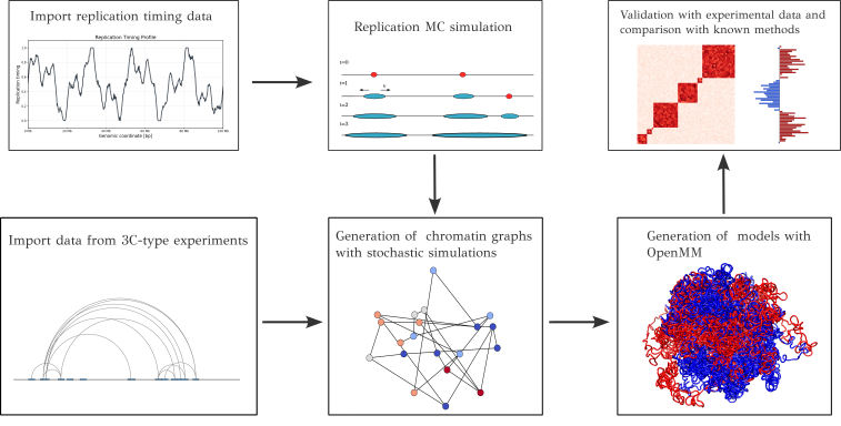
Simulation pipeline
RepliSage is composed by three distinct parts:
Replication simulation (Replikator.py)
This is a simplistic Monte Carlo simulation, where we import single cell replication timing data to model replication. The average replication timing curves can show us the percentage of cells that have been replicated, and from them we estimate the initiation rate $I(x,t)$ which represents the probability fires at time $t$ in loci $x$. Then we employ the Monte Carlo simulation where in each step an origin fires with a probability derived from the initiation rate. When an origin fires, the replication fork start propagating bi-directionally with velocity $v$. The vlocity's mean and standard deviation is derived by calculating the slopes of consecutive optima of the averaged replication timing curve. Replikator outputs the trajectories of the replication forks.
Stochastic simulation that models the interplay of loop extrusion with other factors
In this part we import the previously produced trajectories of replication forks and we model them as moving barriers for the loop extrusion factors. In this way this simulation is composed by three distinct parts:
Loop Extrusion
We use the energy landscape of LoopSage for that. We assume that there are two basic players: LEFs which follow a random difussive motion in 1D and CTCF whose locations are dervied from ChIA-PET data, which are filtered where is a CTCF motif in their sequence. Therefore, assuming that we have $N_{\text{lef}}$ LEFs with two degrees of freedom $(m_i,n_i)$ and epigenetic color states $s_i$ for each monomer, we can write down the following formula,
$$E_{\text{le}} = c_{\text{fold}}\sum_{i=1}^{N_{\text{coh}}}\log(n_i-m_i)+c_{\text{cross}}\sum_{i,j}K(m_i,n_i;m_j,n_j)+c_{\text{bind}}\sum_{i=1}^{N_{\text{coh}}}\left(L(m_i)+R(n_i)\right).$$
In this equation the first term models the folding of chromatin (how fast a loop extrudes, the higher $f$ the more tendency to extrude), the second term is a penalty for cohesin crossing, and the last one minimizes the energy when a LEF encounters a CTCF.
Compartmentalization
It is modelled by using a five stats ($s_i\in[-2,-1,0,1,2]$) Potts model
$$E_{\text{potts}} = C_{p,1} \sum_{k} \left(\dfrac{h_k + h_{t_{r} k}}{2} \right) s_k +C_{p,2}\sum_{i>j} J_{ij}| s_i - s_j |.$$
The second term includes the interaction matrix $J_{ij}$, which is 1 when there is a LEF connecting $i$ with $j$ and 0 if not. The other term represents an epigeetic field. There is an averaged term $h_k$, which represents the averaged replication timing, and a time dependent term $h_{t_{r} k}$ which represents the spread of the epigenetic state due to a single replication fork.
Replication
This term models the interaction between the LEFs and replication forks, $$E_{\text{rep}}=C_{\text{rep}}\sum_{i=1}^{N_{lef}} \mathcal{R}(m_i,n_i ;f_{\text{rep}})$$ and in general penalizes inapropriate configurations between LEFs and replication forks (read the paper).
Therefore, the stochastic simulation integrates the sum of these energies $E = E_{le}+E_{rep}+E_{potts}$ and uses MCMC Metropolis method.
Molecular Dynamics
This parts takes as input the states produced by the stochastic simulation and outputs 3D structures by using a potential in OpenMM. The molecular modeling approach assumes two molecular chains, each consisting of $N_{\text{beads}}$ monomers, where $N_{\text{beads}}$ reflects the granularity of the stochastic simulation. The total potential governing the system is expressed as: $$U = U_{\text{bk}} + U_{\text{le}}(t) + U_{\text{rep}}(t) + U_{\text{block}}(t)$$, where each term corresponds to a specific contribution. The backbone potential ($U_{\text{bk}}$) includes strong covalent bonds between consecutive beads, angular forces, and excluded volume effects to maintain chain integrity. The loop-formation potential ($U_{\text{le}}$) is a time-dependent term introducing harmonic bonds to model loop formation. These bonds are weaker than the backbone interactions and act between dynamically changing pairs of beads, $m_i(t)$ and $n_i(t)$. The last term models compartmentalization with block-copolymer potential.
For more details of the implementation, we suggest to our users to read the method paper of RepliSage.
Requirements
RepliSage is a computationally and biophysically demanding project. It requires significant computing resources, both CPU and GPU. We recommend running RepliSage on high-performance workstations or HPC clusters equipped with a strong CPU and a GPU supporting CUDA (preferred) or at least OpenCL.
RepliSage is tested and supported on Debian-based Linux distributions.
Please note that even on powerful hardware, simulating a full cell cycle for a single chromosome with a polymer of 10,000 beads can take several hours to over a day. While the installation process is straightforward and thoroughly documented in our manual, running simulations will require patience and proper resources.
Installation
It is needed to have at least python 3.10 and run,
pip install -r requirements.txt
Or more easily (do not forget to install it with python 3.10 or higher),
pip install pyRepliSage
How to use?
The usage is very simple. To run this model you need to specify the parameters and the input data. Then RepliSage can do everything for you.
Note that to run replisage it is needed to have GM12878_single_cell_data_hg37.mat data, for single-cell replication timing. These data are not produced by our laboratory, but they are alredy published in the paper of D. S. Massey et al. Please do not forget to cite them. We have uploaded the input data used in the paper here: https://drive.google.com/drive/folders/1PLA147eiHenOw_VojznnlC_ZywhLzGWx?usp=sharing.
Input Data
Replication Timing Data
Single-cell replication timing data are imported automatically in RepliSage (into the directory RepliSage/data),
therefore it is not necessary to prepare them manually. However, in case you would like to use your own data, RepliSage understands Parquet format (for high compression).
Example structure of the expected Parquet data in SC_REPT_PATH:
   chromosome   start     end   center  SC_1  SC_2  SC_3
0           1       0   20000    10000   1.0  NaN   2.0
1           1   20000   40000    30000   3.0  2.0   4.0
Each SC_# column corresponds to a single-cell replication state in the specified genomic window.
From these replication timing data, compartmentalization is also determined, thus it is not required to run any separate compartment caller.
Alternativelly, the user can provide classical averaged replication timing curves in REPT_PATH. The truth is that the single-cell experiment does not add any significant information, and thus the user is free to choose the format they prefer.
The averaged replication timing data should be in txt format and look like this,
Chr 	 Coordinate 	 Replication Timing
1	10257	-0.7371
1	15536	-0.6772
1	17346	-0.6566
1	30810	-0.5037
1	54126	-0.2384
1	57466	-0.2003
1	61854	-0.1502
1	67222	-0.0887
1	95431	0.236
1	100750	0.2976
1	103105	0.3249
1	107644	0.3776
1	109329	0.3972
1	112556	0.4348
1	115568	0.4698
Loop interactions
The main assumption of this work is that the process of replication provides information about compartmentalization and epigenetic mark spreading, since replication timing is highly correlated with compartmentalization, and compartmentalization itself emerges as a macrostate of many interacting epigenetic domains following block-copolymer physics.
However, it is important that the user would specify a .bedpe file with loops. Therefore, in this case RepliSage follows a similar approach like LoopSage and the .bedpe file must be in the following format,
chr1	903917	906857	chr1	937535	939471	16	3.2197903072213415e-05	0.9431392038374097
chr1	979970	987923	chr1	1000339	1005916	56	0.00010385804708107556	0.9755733944997329
chr1	980444	982098	chr1	1063024	1065328	12	0.15405319074060866	0.999801529750033
chr1	981076	985322	chr1	1030933	1034105	36	9.916593137693526e-05	0.01617512105347667
chr1	982171	985182	chr1	990837	995510	27	2.7536240913152036e-05	0.5549511180231224
chr1	982867	987410	chr1	1061124	1066833	71	1.105408615726611e-05	0.9995462969421808
chr1	983923	985322	chr1	1017610	1019841	11	1.7716275555648395e-06	0.10890923034907056
chr1	984250	986141	chr1	1013038	1015474	14	1.7716282101935205e-06	0.025665007111095667
chr1	990949	994698	chr1	1001076	1003483	34	0.5386388489931403	0.9942742844900859
chr1	991375	993240	chr1	1062647	1064919	15	1.0	0.9997541297643132
where the last two columns represent the probabilites for left and right anchor respectively to be tandem right. If the probability is negative it means that no CTCF motif was detected in this anchor. You can extract these probabilities from the repo: https://github.com/SFGLab/3d-analysis-toolkit, with find_motifs.py file. Please set probabilistic=True statistics=False.
Python API
from RepliSage.stochastic_model import *

# Set parameters
N_beads, N_lef, N_lef2 = 1000, 100, 20
N_steps, MC_step, burnin, T, T_min, t_rep, rep_duration = int(8e4), int(4e2), int(1e3), 1.6, 1.0, int(1e4), int(2e4)

f, f2, b, kappa= 1.0, 5.0, 1.0, 1.0
c_state_field, c_state_interact, c_rep = 2.0, 1.0, 1.0
mode, rw, random_spins, rep_fork_organizers = 'Metropolis', True, True, True
Tstd_factor, speed_scale, init_rate_scale, p_rew = 0.1, 20, 1.0, 0.5
save_MDT, save_plots = True, True

# Define data and coordinates
region, chrom =  [80835000, 98674700], 'chr14'

# Data
bedpe_file = '/home/skorsak/Data/method_paper_data/ENCSR184YZV_CTCF_ChIAPET/LHG0052H_loops_cleaned_th10_2.bedpe'
rept_path = '/home/skorsak/Data/Replication/sc_timing/GM12878_single_cell_data_hg37.mat'
out_path = '/home/skorsak/Data/Simulations/RepliSage_whole_chromosome_14'

# Run simulation
sim = StochasticSimulation(N_beads, chrom, region, bedpe_file, out_path, N_lef, N_lef2, rept_path, t_rep, rep_duration, Tstd_factor, speed_scale, init_rate_scale)
sim.run_stochastic_simulation(N_steps, MC_step, burnin, T, T_min, f, f2, b, kappa, c_rep, c_state_field, c_state_interact, mode, rw, p_rew, rep_fork_organizers, save_MDT)
if show_plots: sim.show_plots()
sim.run_openmm('OpenCL',mode='MD')
if show_plots: sim.compute_structure_metrics()

# Save Parameters
if save_MDT:
    params = {k: v for k, v in locals().items() if k not in ['args','sim']}
    save_parameters(out_path+'/other/params.txt',**params)
Bash command
An even easier way that you can avoid all python coding is by running the command,
replisage -c config.ini
The configuration file has the usual form,
[Main]

; Input Data and Information
BEDPE_PATH = /home/blackpianocat/Data/method_paper_data/ENCSR184YZV_CTCF_ChIAPET/LHG0052H_loops_cleaned_th10_2.bedpe
REPT_PATH = /home/blackpianocat/Data/Replication/sc_timing/GM12878_single_cell_data_hg37.mat
REGION_START = 80835000
REGION_END = 98674700
CHROM = chr14
PLATFORM = CUDA
OUT_PATH = /home/blackpianocat/Data/Simulations/RepliSage_test

; Simulation Parameters
N_BEADS = 2000
N_LEF = 200
BURNIN = 1000
T_INIT = 1.8
T_FINAL = 1.0
METHOD = Metropolis
LEF_RW = True
RANDOM_INIT_SPINS = True

; Molecular Dynamics
INITIAL_STRUCTURE_TYPE = rw
SIMULATION_TYPE = MD
TOLERANCE = 1.0
EV_P=0.01
You can define these parameters based on the table of simulation parameters.
Parameter table
General Settings
| Parameter Name | Type | Default Value | Description |
|---|---|---|---|
| PLATFORM | str | CPU | Specifies the computational platform to use (e.g., CPU, CUDA). |
| DEVICE | str | None | Defines the specific device to run the simulation (e.g., GPU ID). |
| OUT_PATH | str | ../results | Directory where simulation results will be saved. |
| SAVE_PLOTS | bool | True | Enables saving of simulation plots. |
| SAVE_MDT | bool | True | Enables saving of molecular dynamics trajectories. |
| VIZ_HEATS | bool | True | Enables visualization of heatmaps. |
Input Data
| Parameter Name | Type | Default Value | Description |
|---|---|---|---|
| BEDPE_PATH | str | None | Path to the BEDPE file containing CTCF loop data. |
| SC_REPT_PATH | str | defailt_rept_path |
Path to the single cell replication timing data file. |
| REPT_PATH | str | None | Path to the replication timing data file. If specified, it does not take SC_REPT_PATH into account. |
| REGION_START | int | None | Start position of the genomic region to simulate. |
| REGION_END | int | None | End position of the genomic region to simulate. |
| CHROM | str | None | Chromosome identifier for the simulation. |
Simulation Parameters
| Parameter Name | Type | Default Value | Description |
|---|---|---|---|
| N_BEADS | int | None | Number of beads in the polymer chain. |
| N_LEF | int | None | Number of loop extrusion factors (LEFs). |
| N_LEF2 | int | 0 | Number of secondary loop extrusion factors. |
| COHESIN_BLOCKS_CONDENSIN | bool | False | Enables a feature where cohesin blocks condensin activity during G2/M phase. |
| LEF_RW | bool | True | Enables random walk for loop extrusion factors (LEFs). |
| LEF_DRIFT | bool | False | Enables drift for loop extrusion factors. |
| RANDOM_INIT_SPINS | bool | True | Randomizes initial Potts model spin states. |
| REP_WITH_STRESS | bool | False | Enables a helper to set parameters for modeling replication stress. Overrides user-defined REP_T_STD_FACTOR, REP_SPEED_SCALE, and REP_INIT_RATE_SCALE. |
| REP_START_TIME | int | 50000 | Start time for replication in simulation steps. |
| REP_TIME_DURATION | int | 50000 | Duration of the replication process in simulation steps. |
| REP_T_STD_FACTOR | float | 0.1 | Standard deviation factor for replication timing. |
| REP_SPEED_SCALE | float | 20 | Scaling factor for replication fork speed. |
| REP_INIT_RATE_SCALE | float | 1.0 | Scaling factor for replication initiation rate. |
| N_STEPS | int | 200000 | Total number of simulation steps. |
| N_SWEEP | int | 1000 | Number of proposed moves per step. |
| MC_STEP | int | 200 | Number of steps per Monte Carlo iteration. |
| BURNIN | int | 1000 | Number of burn-in steps before data collection. |
| T_MC | float | 1.5 | Order parameter or "temperature" of Metropolis-Hastings. |
Stochastic Energy Coefficients
| Parameter Name | Type | Default Value | Description |
|---|---|---|---|
| FOLDING_COEFF | float | 1.0 | Coefficient controlling chromatin folding. |
| FOLDING_COEFF2 | float | 0.0 | Secondary coefficient for chromatin folding. |
| REP_COEFF | float | 1.0 | Coefficient for replication-related energy terms. |
| POTTS_INTERACT_COEFF | float | 1.0 | Coefficient for Potts model interaction energy. |
| POTTS_FIELD_COEFF | float | 1.0 | Coefficient for Potts model field energy. |
| CROSS_COEFF | float | 1.0 | Coefficient penalizing LEF crossing. |
| BIND_COEFF | float | 1.0 | Coefficient for LEF binding energy. |
Molecular Dynamics
| Parameter Name | Type | Default Value | Description |
|---|---|---|---|
| INITIAL_STRUCTURE_TYPE | str | rw | Type of initial structure (e.g., rw for random walk). |
| SIMULATION_TYPE | str | None | Type of simulation to run (e.g., MD or EM). |
| DCD_REPORTER | bool | False | Enables saving of molecular dynamics trajectories in DCD format. |
| INTGRATOR_TYPE | str | langevin | Type of integrator for molecular dynamics. |
| INTEGRATOR_STEP | Quantity | 10 femtosecond | Time step for the molecular dynamics integrator. |
| FORCEFIELD_PATH | str | default_xml_path | Path to the force field XML file. |
| EV_P | float | 0.01 | Excluded volume parameter for molecular dynamics. |
| TOLERANCE | float | 1.0 | Tolerance for energy minimization. |
| SIM_TEMP | Quantity | 310 kelvin | Temperature for molecular dynamics simulation. |
| SIM_STEP | int | 10000 | Number of steps for molecular dynamics simulation. |
Output and Results
The output is organized into a well-structured directory hierarchy as follows:
.
├── ensemble
│   ├── ensemble_10_BR.cif
│   ├── ensemble_11_BR.cif
│   ├── ensemble_12_BR.cif
│   ├── ensemble_13_BR.cif
├── metadata
│   ├── energy_factors
│   │   ├── Bs.npy
│   │   ├── Es.npy
│   │   ├── Es_potts.npy
│   │   └── Fs.npy
│   ├── graph_metrics
│   ├── MCMC_output
│   │   ├── loop_lengths.npy
│   │   ├── mags.npy
│   │   ├── Ms.npy
│   │   ├── Ns.npy
│   │   └── spins.npy
│   ├── md_dynamics
│   │   ├── LE_init_struct.cif
│   │   ├── minimized_model.cif
│   │   └── replisage.psf
│   └── structural_metrics
└── plots
    ├── graph_metrics
    ├── MCMC_diagnostics
    ├── replication_simulation
    │   ├── rep_frac.png
    │   └── rep_simulation.png
    └── structural_metrics
└── params.txt
Directory Details
-
ensemble: Stores 3D structural ensembles categorized by cell cycle phase:G1: Structures representing the pre-replication phase (with BR, before replication).S: Structures captured during the replication phase (with R during replication).G2M: Structures corresponding to the post-replication phase (with AR after replication).
-
metadata: Contains simulation data and intermediate outputs:energy_factors: Numerical arrays for energy components (e.g., folding, Potts model).graph_metrics: Graph-related metrics such as clustering coefficients and degree distributions.MCMC_output: Results from the Monte Carlo simulation, including loop lengths and spin states.md_dynamics: Files for molecular dynamics visualization (e.g.,.psf,.cif).structural_metrics: Structural properties like radius of gyration and contact probabilities.
-
plots: Includes visualizations and diagnostic plots:graph_metrics: Graph-related metric plots (e.g., clustering coefficients).MCMC_diagnostics: Diagnostics for the MCMC algorithm (e.g., autocorrelation).replication_simulation: Visualizations of replication dynamics.structural_metrics: Plots of structural properties (e.g., radius of gyration).
This directory structure ensures clear organization and facilitates efficient analysis of results, with data neatly separated by phase and type.
params.txt file contains information about the input parameters.
Expected Results
Averaged loop diagram
RepliSage aims to model a very biophysically complex process: the cell-cycle. Because of that the results are very sensitive in the input parameters. Therefore, it is important to be able to understand the diagnostic plots, so as to be able to distinguish if the model's result have a biophysical meaning or not.
One of the most important diagnostic plots is the diagram of average loop length as a function of time (with decision intervals),
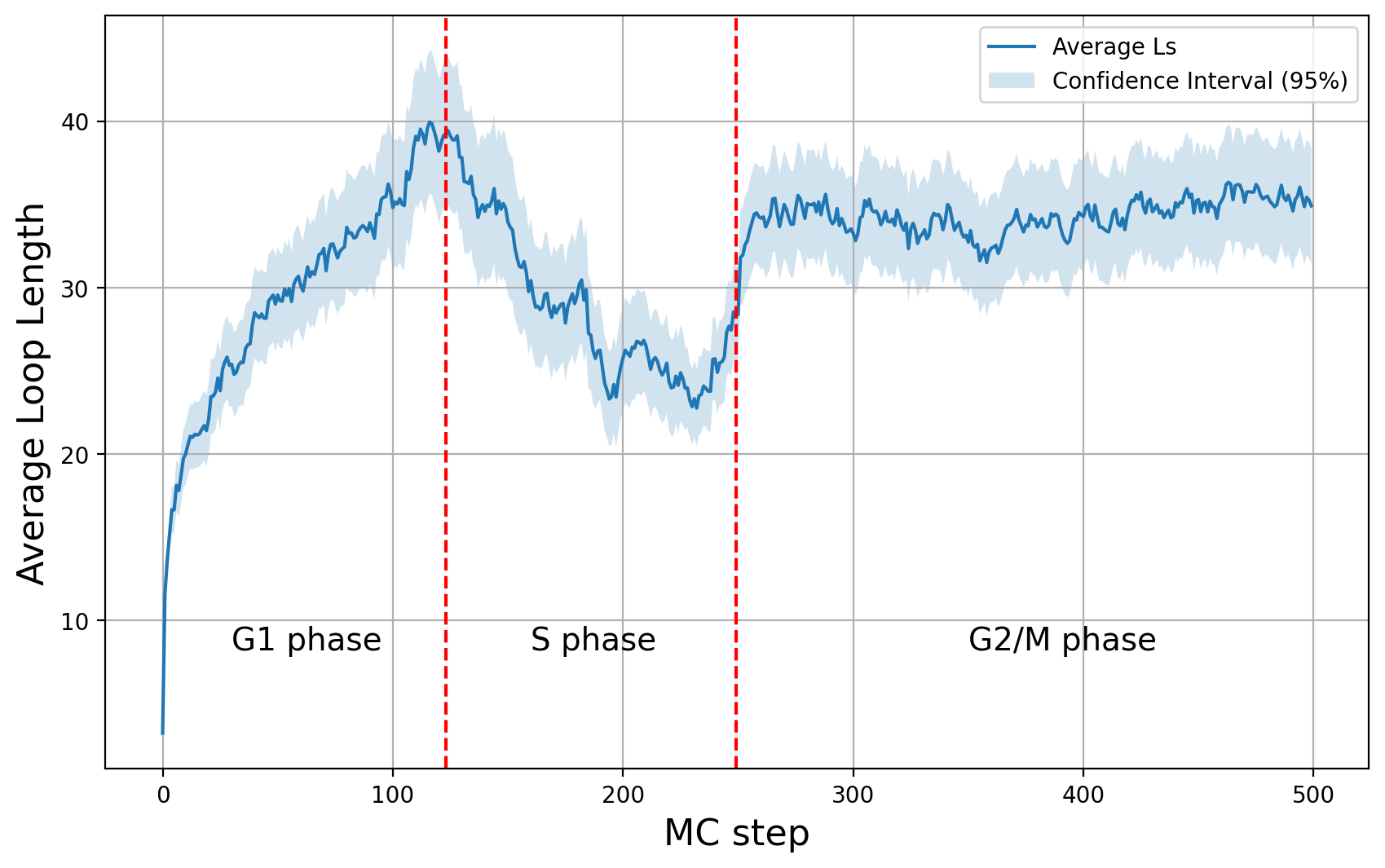
This plot shows us a very clear biophysical behavior:
- The simulation initially reaches the equillibrium in G1 phase.
- In S phase the average loop length is getting smaller because of the barrier activity of replication forks. This is a result which is also expected experimentally, as it is observed that during replication there is tendency that loops are getting shorter.
- After replication, in G2/M phase, condensins come into the game and they extrude loops faster. This means during this phase we excpect a different average loop length in equillibrium.
This is a very good plot, because we can see if there is equilibrium. In the previous example, we can see that the simulation reaches the equilibrium in G2/M phase. However, during G1 phase, maybe we should make more Monte Carlo steps so as to have more ensembles in equilibrium. S phase should always be out of equillibrium, but it is important to have enough steps for this phase as well, because replication forks are considered to be much slower than LEFs.
State Diagram
Here we have a different type of diagram, which combime node states and link states of ou co-evolutionary network. In this plot, we draw the percentage of links that connect the same node states (you can think of them as epigenetic states or compartments), and the percentage of links that connect different node states.
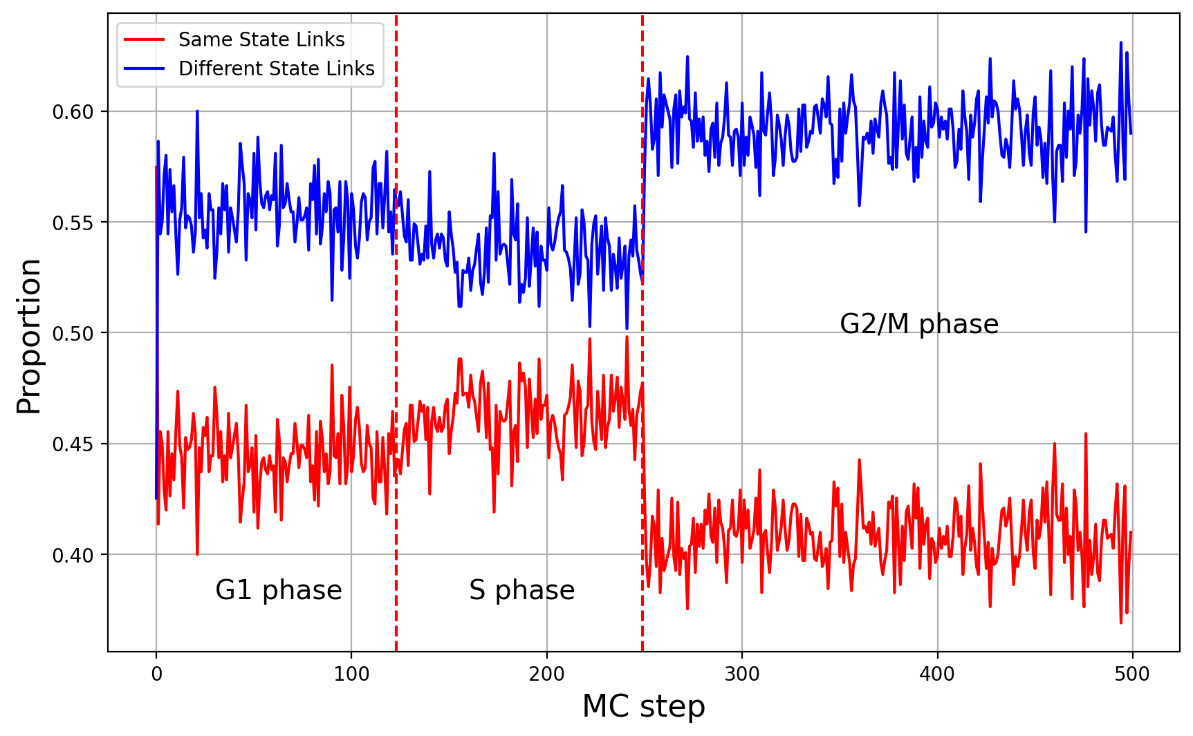
What is this diagram showing us
- There is a small increase in links with the same node state during S phase. This is good because, Peano et al. observed similar behavior experimentally.
- In G2/M phase we have sudden decrease of the links that connect the same node state. This can be because during mitosis, condensins extrude long loops and loop extrusion wins over compartmentalization. In general, this result might be different depending of the parameters of
N_lef2(number of condensins in G2/M phase) or their folding coefficient.
From this plot we can see that there is equillibrium in node states in each phase (also important).
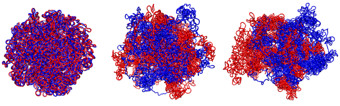
Structural metrics
Previous two metrics were connected with the states of our graph, but they did not touch at all a very important aspect of modelling: the 3D structure. This is the reason why RepliSage outputs a set of sructural metrics as well. For example,
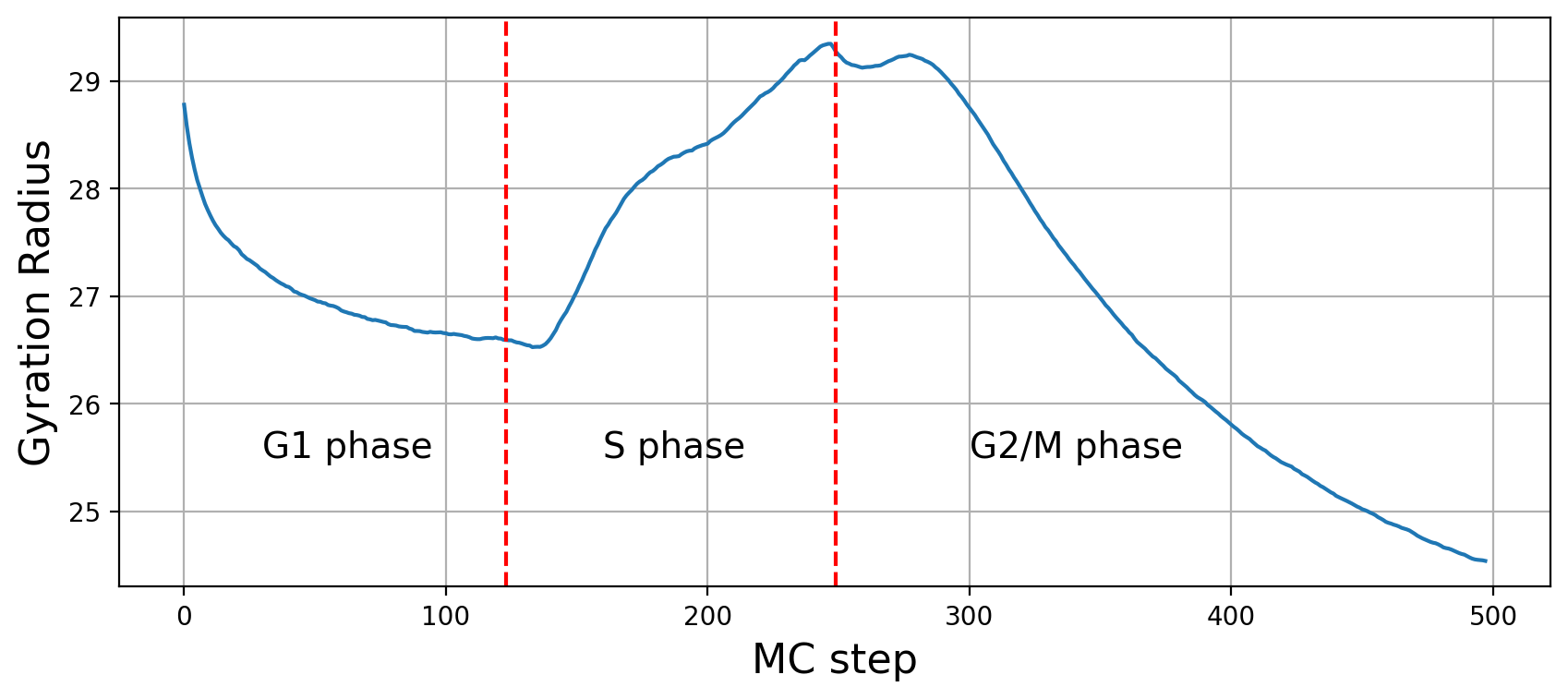
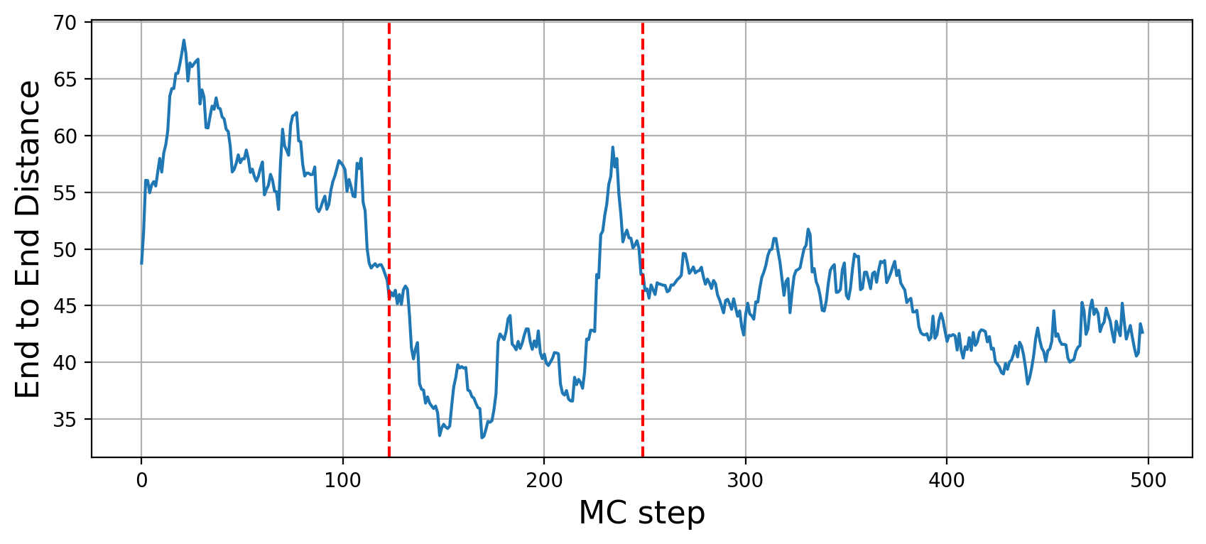
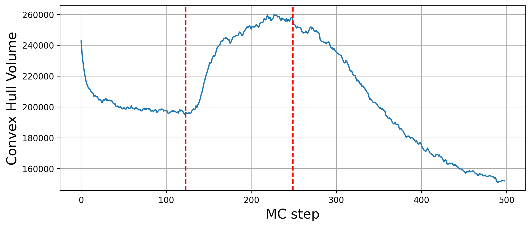
These plots show us that during S phase replication forks are detaching the two replicates from each other. This effect in combination to the excluded volume causes less compacted structure. After S phase, in G2/M phase there is further compactions due to the interplay of: excluded volume, block-copolymer forces and long range condensin loops.
Citation
Please cite the preprint of our paper in case of usage of this software
- S. Korsak et al, Chromatin as a Coevolutionary Graph: Modeling the Interplay of Replication with Chromatin Dynamics, bioRxiv, 2025-04-04
- D. J. Massey and A. Koren, “High-throughput analysis of single human cells reveals the complex nature of dna replication timing control,” Nature Communications, vol. 13, no. 1, p. 2402, 2022.
Release history Release notifications | RSS feed


Download files
Download the file for your platform. If you're not sure which to choose, learn more about installing packages.
Source Distribution
Built Distribution
Filter files by name, interpreter, ABI, and platform.
If you're not sure about the file name format, learn more about wheel file names.
Copy a direct link to the current filters
File details
Details for the file pyreplisage-0.2.0.tar.gz.
File metadata
- Download URL: pyreplisage-0.2.0.tar.gz
- Upload date:
- Size: 7.4 MB
- Tags: Source
- Uploaded using Trusted Publishing? No
- Uploaded via: twine/6.1.0 CPython/3.8.20
File hashes
| Algorithm | Hash digest | |
|---|---|---|
| SHA256 |
e1ae01b88655bfc24eb22b4a0d79c7363f2b0d3fd09a8a4b920f1a59195ce15a
|
|
| MD5 |
d3f197bac48f2541fda1ad64a21bd2f7
|
|
| BLAKE2b-256 |
0ab21e5ee38b209f743335982058d054bedcc16b99fa3b1ae2d1bfc85f0060ab
|
File details
Details for the file pyreplisage-0.2.0-py3-none-any.whl.
File metadata
- Download URL: pyreplisage-0.2.0-py3-none-any.whl
- Upload date:
- Size: 7.4 MB
- Tags: Python 3
- Uploaded using Trusted Publishing? No
- Uploaded via: twine/6.1.0 CPython/3.8.20
File hashes
| Algorithm | Hash digest | |
|---|---|---|
| SHA256 |
e461c4090ba9846a0b09aa0bb1051c8ea09df3df84a11ad932551ea054b6e42c
|
|
| MD5 |
454e5c9b8b4ab82a957733ea76469eeb
|
|
| BLAKE2b-256 |
c9c5ad80af139002694ae033084f337e9e6a96f49c770bcaba73d8757151f2ce
|


