Fast multi-dimensional Chebyshev tensor interpolation with analytical derivatives
Verified details
These details have been verified by PyPIProject links
GitHub Statistics
Maintainers

Project description
PyChebyshev


A fast Python library for multi-dimensional Chebyshev tensor interpolation with analytical derivatives
PyChebyshev provides a fully optimized Python implementation of the Chebyshev tensor method, demonstrating that it achieves comparable speed and accuracy to the state-of-the-art MoCaX C++ library for European option pricing via Black-Scholes — with pure Python and NumPy only.
Performance Comparison
Based on standardized 5D Black-Scholes tests (test_5d_black_scholes() with S, K, T, σ, r):
| Method | Price Error | Greek Error | Build Time | Query Time | Notes |
|---|---|---|---|---|---|
| Analytical | 0.000% | 0.000% | N/A | ~10μs | Ground truth (blackscholes library) |
| Chebyshev Barycentric | 0.000% | 1.980% | ~0.35s | ~0.065ms | Vectorized NumPy + BLAS reshape trick |
| Chebyshev Baseline | 0.000% | 1.980% | ~0.35s | ~2-3ms | NumPy polynomial basis |
| MoCaX Standard | 0.000% | 1.980% | ~1.04s | ~0.47ms | Proprietary C++, full tensor (161k evals) |
| FDM | 0.803% | 2.234% | N/A | ~0.5s/case | PDE solver, no pre-computation |
Key Insights:
- Chebyshev Barycentric achieves spectral accuracy (0.000% price error, identical to MoCaX)
- Greeks accuracy: 1.98% max error (Vega) via analytical differentiation matrices
- Build time: 0.35s (161,051 analytical evaluations) vs MoCaX 1.04s (C++ overhead)
- Query time: 0.065ms price / 0.29ms price+5 Greeks (vectorized NumPy) vs 0.47ms (MoCaX Standard)
- Break-even: > 1 query makes pre-computation worthwhile
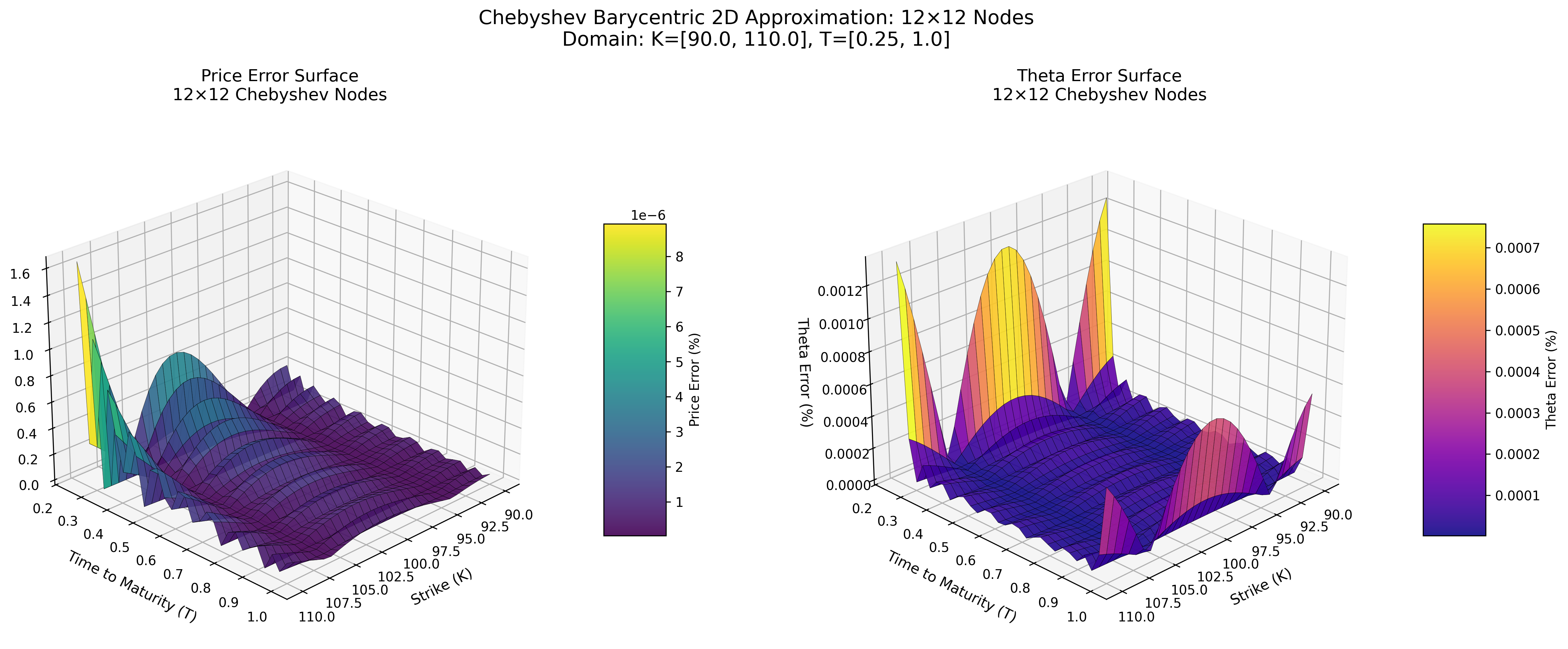
Visual Comparison: Spectral Convergence
Error Surface at 12×12 Nodes
Chebyshev Barycentric (Python)
MoCaX Standard (C++)
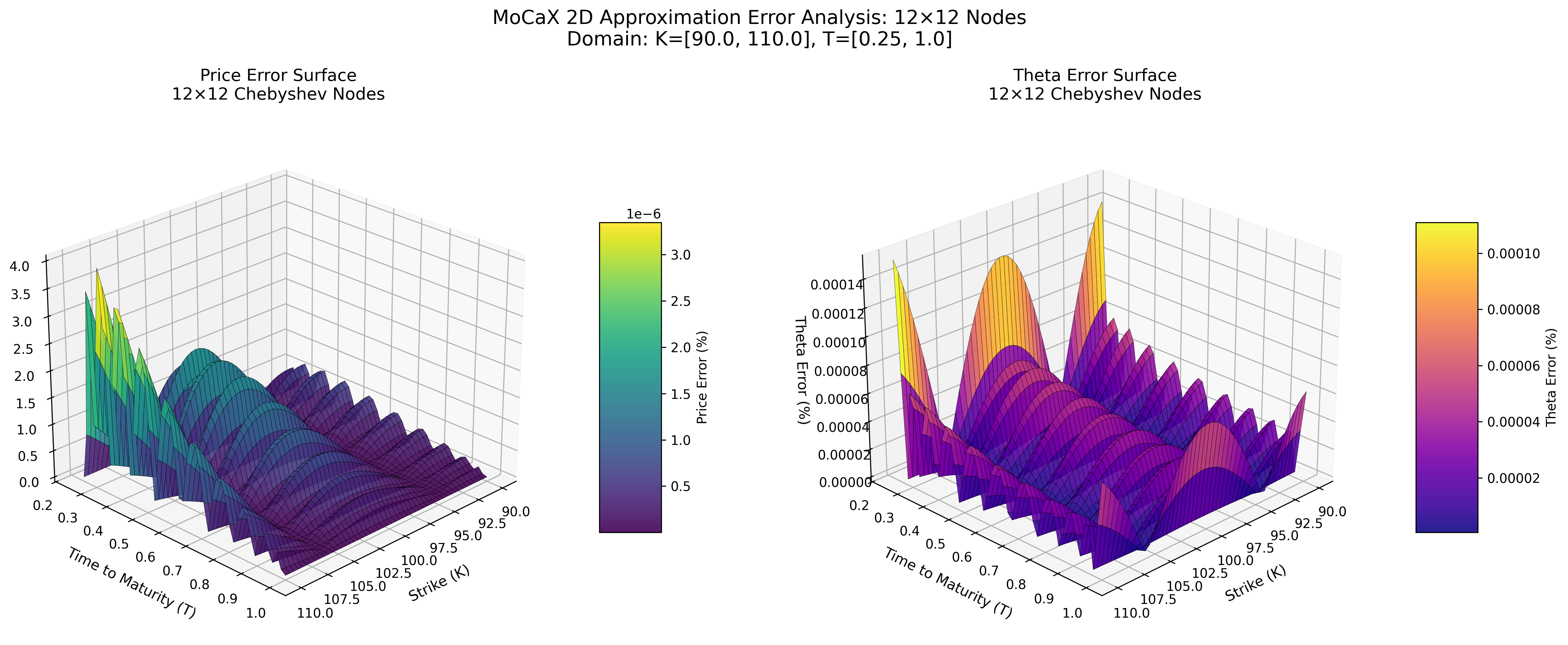
Both methods achieve spectral accuracy (exponential error decay) with identical node configurations, demonstrating that the pure Python implementation successfully replicates the MoCaX algorithm's mathematical foundation.
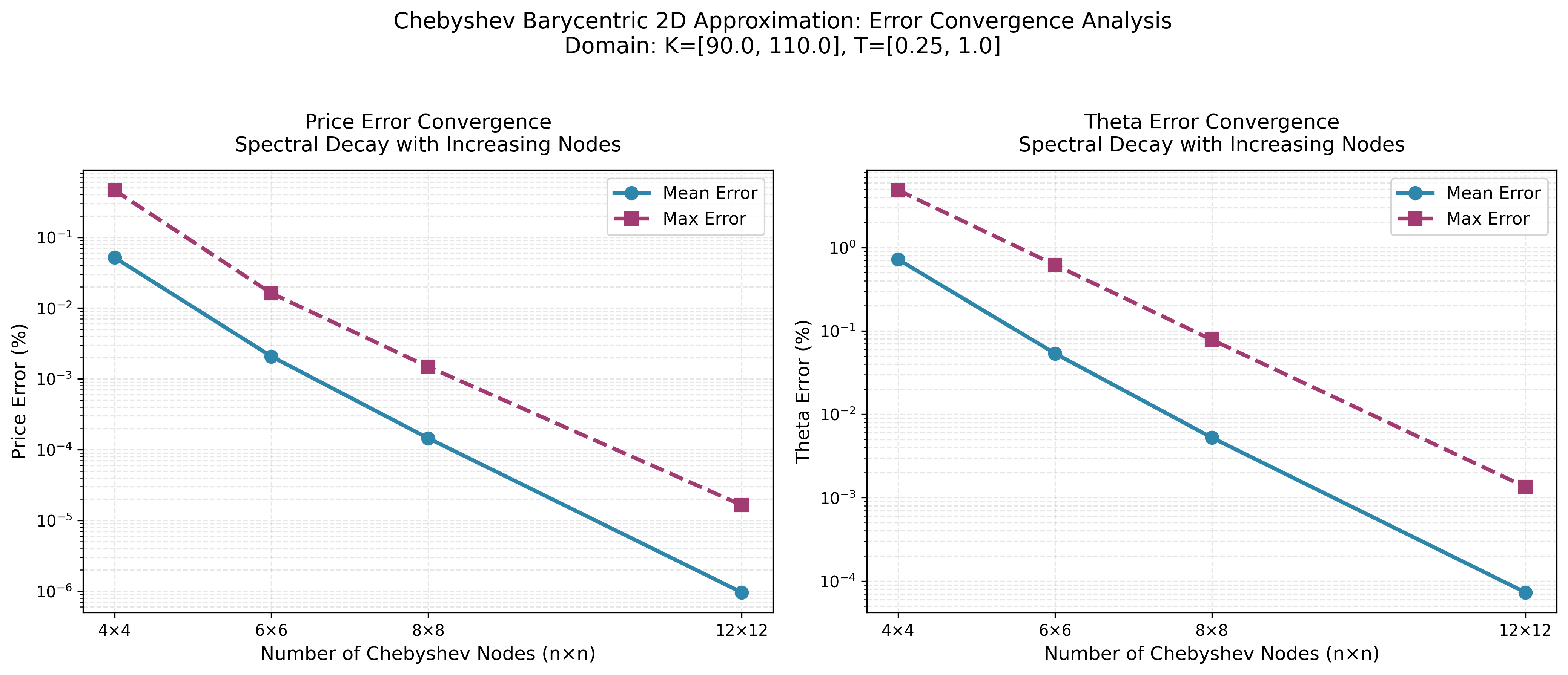
Convergence Analysis
Chebyshev Barycentric
MoCaX Standard
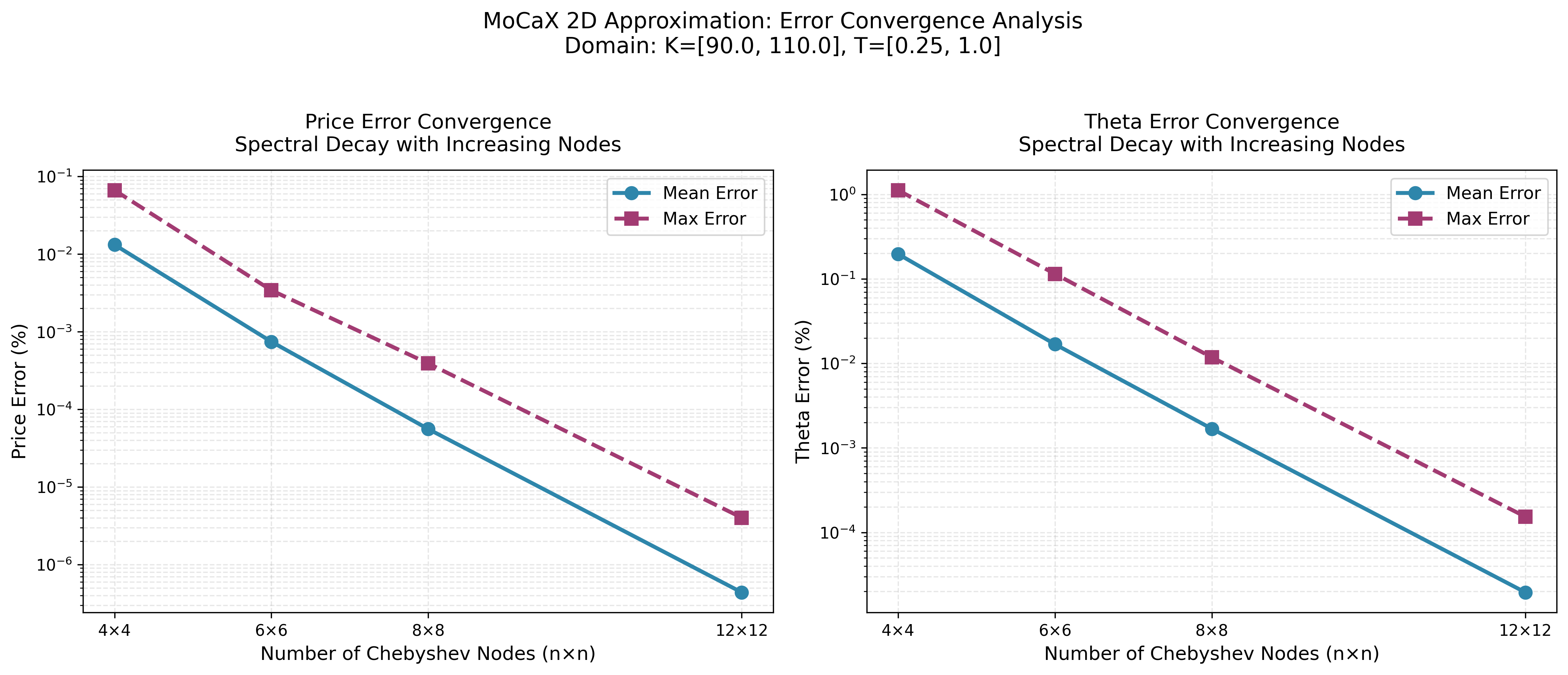
The convergence plots demonstrate exponential error decay as node count increases, confirming the spectral accuracy predicted by the Bernstein Ellipse Theorem. Errors drop rapidly from 4×4 to 12×12 nodes, reaching near-machine precision for this analytic function.
Features
- Full tensor interpolation via
ChebyshevApproximation— spectral accuracy for up to ~5-6 dimensions - Sliding technique via
ChebyshevSlider— additive decomposition for high-dimensional functions (10+ dims) - Analytical derivatives via spectral differentiation matrices (no finite differences)
- Vectorized evaluation using BLAS matrix-vector products (~0.065ms/query)
- Pure Python — NumPy + SciPy only, no compiled extensions needed
Acknowledgments
Special thanks to MoCaX for their high-quality videos on YouTube explaining the mathematical foundations behind their library. These resources were invaluable for understanding and implementing the barycentric Chebyshev interpolation algorithm.
Getting Started
Installation
pip install pychebyshev
Quick Example
import math
from pychebyshev import ChebyshevApproximation

# Approximate any smooth function
def my_func(x, _):
    return math.sin(x[0]) * math.exp(-x[1])

cheb = ChebyshevApproximation(
    my_func,
    num_dimensions=2,
    domain=[[-1, 1], [0, 2]],
    n_nodes=[15, 15],
)
cheb.build()

# Evaluate function value
value = cheb.vectorized_eval([0.5, 1.0], [0, 0])

# Analytical first derivative w.r.t. x[0]
dfdx = cheb.vectorized_eval([0.5, 1.0], [1, 0])

# Price + all derivatives at once (shared weights, ~25% faster)
results = cheb.vectorized_eval_multi(
    [0.5, 1.0],
    [[0, 0], [1, 0], [0, 1], [2, 0]],
)
High-Dimensional Functions (Sliding Technique)
For functions with more than ~6 dimensions, use ChebyshevSlider to decompose into low-dimensional slides:
from pychebyshev import ChebyshevSlider

slider = ChebyshevSlider(
    my_func, num_dimensions=10,
    domain=[[-1, 1]] * 10,
    n_nodes=[11] * 10,
    partition=[[0, 1], [2, 3], [4, 5], [6, 7], [8, 9]],
    pivot_point=[0.0] * 10,
)
slider.build()
val = slider.eval([0.5] * 10, [0] * 10)
See the documentation for full API reference and usage guides.
Technicals
This demonstration uses Chebyshev tensor interpolation to accelerate the calculation of prices and derivatives for European options. The approach generalizes to all analytic functions, as proven by Theorems 2.1 and 2.2 in Gaß et al. (2018), "Chebyshev Interpolation for Parametric Option Pricing", Finance and Stochastics, 22(3), which establish (sub)exponential convergence rates for Chebyshev interpolation of parametric conditional expectations.
Problem Statement
European option pricing requires evaluating a 5-dimensional function:
V = f(S, K, T, σ, r)
where:
- S: Spot price
- K: Strike price
- T: Time to maturity
- σ: Volatility
- r: Risk-free rate
Challenges:
- Analytical formulas are instant but limited to European vanilla options
- Numerical PDE solvers (FDM) are flexible but slow (~0.5s per solve)
- Need to compute Greeks (Delta, Gamma, Vega, Rho, Theta) across diverse scenarios
- Production systems require thousands of evaluations per second
Goal: Pre-compute an approximation that achieves:
- ✅ High accuracy (< 2% error on Greeks)
- ✅ Fast evaluation (< 2ms per query)
- ✅ Support for multi-parameter variation (all 5 dimensions)
Mathematical Foundation
This section establishes the theoretical foundation for Chebyshev interpolation, explaining why it is the appropriate approach and how the mathematics guarantee exceptional performance.
Why Chebyshev Interpolation?
Equally-spaced points appear simpler for polynomial interpolation, but suffer from fundamental limitations discovered by Carl Runge in 1901.
Runge's Phenomenon: When More is Worse
In 1901, Carl Runge demonstrated that polynomial interpolation with equally-spaced points can actually diverge as polynomial degree increases, even for smooth, well-behaved functions (Wikipedia).
Consider Runge's classic example: the function $$f(x) = \frac{1}{1 + 25x^2}$$ on the interval $$[-1, 1]$$. This function is perfectly smooth and analytic everywhere. Interpolating this function with high-degree polynomials using equally-spaced points produces wild oscillations near the endpoints of the interval. Increasing the polynomial degree makes the oscillations worse, not better - the approximation diverges rather than converges.
This phenomenon occurs because equally-spaced nodes lead to a rapidly growing Lebesgue constant (roughly $$O(2^n/n)$$), which amplifies approximation errors, especially near the interval boundaries.
Chebyshev's Solution: Strategic Node Placement
Chebyshev nodes address this issue by using non-uniform spacing:
$$x_i = \cos\left(\frac{(2i-1)\pi}{2n}\right), \quad i=1,\ldots,n$$
These are the roots of the Chebyshev polynomial $$T_n(x)$$, which cluster near the interval boundaries $$x = \pm 1$$ with more spacing in the middle. Since polynomial interpolation errors tend to be largest near endpoints, this clustering compensates for the natural error growth in those regions.
For arbitrary intervals $$[a, b]$$, the Chebyshev nodes are transformed via:
$$\xi_i = \frac{a+b}{2} + \frac{b-a}{2} \cdot x_i$$
Numerical Stability
Beyond avoiding Runge's phenomenon, Chebyshev nodes provide excellent numerical stability. The Lebesgue constant for Chebyshev nodes grows only logarithmically: $$\Lambda_n \leq \frac{2}{\pi}\log(n+1) + 1$$ (Günttner, 1980).
Theoretical Guarantees
Three fundamental theorems guarantee the exceptional performance of Chebyshev interpolation.
Polynomial Uniqueness: A Fundamental Guarantee
A fundamental result from numerical analysis states that for any $$n+1$$ distinct points $$(x_0, y_0), (x_1, y_1), \ldots, (x_n, y_n)$$, there exists exactly one polynomial $$p(x)$$ of degree at most $$n$$ such that $$p(x_i) = y_i$$ for all $$i = 0, 1, \ldots, n$$.
This is known as the Polynomial Interpolation Uniqueness Theorem (Wikipedia: Polynomial Interpolation). This guarantees that Chebyshev interpolants through $$n+1$$ function values at Chebyshev nodes produce a well-defined, unique polynomial with no computational ambiguity.
This uniqueness holds regardless of how we compute the polynomial (Lagrange form, Newton form, barycentric form) - they all produce the same result, just through different computational paths.
Convergence Rate: Interpolation vs. Best Approximation
Polynomial interpolation (matching function values at specific points) can be compared to the best possible polynomial approximation (minimizing the maximum error over the entire interval). Two approaches exist for approximating $$f(x)$$ with a polynomial $$p_n(x)$$ of degree $$n$$:
-
Chebyshev projection (also called "best approximation"): Find the polynomial $$f_n$$ that minimizes
$$|f - f_n|_\infty = \max_{x \in [-1,1]} |f(x) - f_n(x)|$$
This is theoretically optimal, but requires solving an optimization problem.
-
Chebyshev interpolation (used in this work): Build a polynomial $$p_n$$ that matches $$f$$ exactly at the $$n+1$$ Chebyshev nodes. This is computationally simple - evaluate $$f$$ at the nodes and apply the interpolation formula.
Lloyd Trefethen's analysis (Trefethen, "Approximation Theory and Approximation Practice", Chapter 4, SIAM 2019) establishes that for functions analytic in a Bernstein ellipse with parameter $$\rho > 1$$, both methods achieve essentially the same exponential convergence rate:
- Chebyshev projection: $$|f - f_n|_\infty \leq \frac{2M\rho^{-n}}{\rho-1}$$
- Chebyshev interpolation: $$|f - p_n|_\infty \leq \frac{4M\rho^{-n}}{\rho-1}$$
The bounds differ only by a constant factor of 2. Both achieve the same exponential convergence rate $$O(\rho^{-n})$$, meaning interpolation-based methods are essentially as good as theoretically optimal approximations - at most one bit of accuracy is lost compared to best polynomial approximation.
The practical implication: simple, fast interpolation approaches achieve nearly optimal results without requiring complex optimization algorithms.
Spectral Convergence: Exponential Error Decay
The 2D error surface plots (12×12 nodes showing 0.0000% errors) demonstrate spectral convergence - accuracy improving dramatically with additional nodes.
The Bernstein Ellipse Theorem, established by Sergey Bernstein in 1912 (Trefethen, "Approximation Theory and Approximation Practice", Chapter 8, SIAM 2019), provides the theoretical explanation:
Theorem: If a function $$f(x)$$ is analytic and bounded in a Bernstein ellipse with parameter $$\rho > 1$$, then the Chebyshev interpolation error decays geometrically:
$$|f(x) - p_N(x)| = O(\rho^{-N})$$
A Bernstein ellipse is an ellipse in the complex plane with foci at $$x = -1$$ and $$x = +1$$. The parameter $$\rho$$ equals the sum of the ellipse's semimajor and semiminor axis lengths. Larger ellipses (where the function remains analytic without singularities, poles, or branch cuts) correspond to larger $$\rho$$ and faster error decay.
Exponential decay means each additional node reduces error by a constant factor $$\rho$$, not a constant amount. This spectral accuracy causes errors to drop to machine precision rapidly.
Two Implementation Approaches
With the theoretical foundation established, Chebyshev interpolation can be implemented via different computational paths. The Uniqueness Theorem guarantees a single polynomial through the data points, but multiple computational representations exist. We explore two approaches:
-
Polynomial Coefficients Approach (Baseline): Express $$p(x) = \sum_{k=0}^{n} c_k T_k(x)$$ where $$T_k$$ are Chebyshev polynomials. Compute coefficients $$c_k$$ from function values. Simple and uses NumPy's built-in tools, but has a limitation for multi-dimensional pre-computation.
-
Barycentric Weights Approach (Our Implementation): Use the barycentric interpolation formula with pre-computed weights $$w_i$$. This enables full pre-computation across all dimensions, and analytic derivative taking in any direction, resulting in significant speedups.
Method 1: Chebyshev Baseline (Polynomial Coefficients)
Benchmark script: chebyshev_baseline.py
Dimensional Decomposition Strategy
The straightforward implementation of multi-dimensional Chebyshev interpolation uses dimensional decomposition. Given a 5D function $$V(S, K, T, \sigma, r)$$ evaluated at $$11^5 = 161,051$$ Chebyshev nodes, evaluating at an off-grid point like $$V(100, 100, 1.0, 0.25, 0.05)$$ requires breaking the 5D interpolation into sequential 1D interpolations rather than attempting direct 5D interpolation.
Decomposition Process
The evaluation proceeds by sequential dimensional collapse:
Initial state: 5D tensor $$V[i_S, i_K, i_T, i_\sigma, i_r]$$ with indices 0-10 (11 nodes per dimension).
Collapse sequence:
- Fix $$r$$: Interpolate along $$r$$ dimension at $$r = 0.05$$ for all $$(S, K, T, \sigma)$$ combinations → 4D tensor
- Fix $$\sigma$$: Interpolate along $$\sigma$$ dimension at $$\sigma = 0.25$$ for all $$(S, K, T)$$ combinations → 3D tensor
- Fix $$T, K, S$$: Continue interpolating each dimension sequentially → final scalar
Mathematically:
- 5D → 4D: Interpolate $$r$$
- 4D → 3D: Interpolate $$\sigma$$
- 3D → 2D: Interpolate $$T$$
- 2D → 1D: Interpolate $$K$$
- 1D → scalar: Interpolate $$S$$
Polynomial Coefficient Representation
Each 1D interpolation step computes a polynomial through 11 Chebyshev nodes using NumPy's Chebyshev.interpolate(), which represents the polynomial in Chebyshev basis form:
$$p(x) = \sum_{k=0}^{10} c_k T_k(x)$$
where $$T_k(x)$$ are Chebyshev polynomials of the first kind and $$c_k$$ are coefficients. The Chebyshev basis provides numerical stability, and coefficients are computed via FFT-based algorithms in $$O(N \log N)$$ time. Once coefficients are determined, evaluating $$p(x)$$ is efficient.
Pre-computation Limitation
The critical question: can we pre-compute ALL polynomial coefficients for all dimensions?
Answer: only partially.
During dimensional decomposition:
-
Innermost dimension ($$S$$ in our case): The "function values" here are the actual option prices we evaluated at build time. These are known constants. So we can pre-compute $$11^4 = 14,641$$ polynomial objects (one for each combination of $$K, T, \sigma, r$$) and store them.
-
Outer dimensions ($$K, T, \sigma, r$$): The "function values" here are NOT the original option prices - they're intermediate results from the previous interpolation step! These depend on where we're querying, so we can't know them ahead of time.
Fundamental constraint: polynomial coefficients $$c_k$$ depend on BOTH node positions $$x_i$$ (known at build time) AND function values $$f_i$$ (for outer dimensions, these are query-dependent intermediate results).
Implication: polynomials for the outer 4 dimensions must be recomputed during each query. Full pre-computation is impossible with this representation.
Python Implementation
The dimensional decomposition translates to:
# Build phase: Pre-compute polynomials for innermost dimension only
class ChebyshevApproximation:
    def __init__(self, func, domain, num_nodes_per_dim):
        # Evaluate function at all 11^5 Chebyshev nodes
        self.tensor = self._build_tensor(func, domain, num_nodes_per_dim)

        # Pre-compute polynomial objects for innermost dimension
        # This gives us 11^4 = 14,641 Chebyshev polynomial objects
        self.innermost_polys = {}
        for idx in product(range(11), repeat=4):  # All combos of K,T,σ,r
            values = self.tensor[..., idx[0], idx[1], idx[2], idx[3]]
            self.innermost_polys[idx] = Chebyshev.interpolate(
                lambda x: values,
                deg=10,
                domain=domain[0]
            )

    def eval(self, point):
        # Query phase: Dimensional collapse 5D → 4D → 3D → 2D → 1D → scalar
        S, K, T, sigma, r = point

        # Step 1: Interpolate r (outermost) - must recompute polynomial!
        temp_4d = self._interpolate_dimension(self.tensor, r, dim=4)

        # Step 2: Interpolate σ - must recompute polynomial!
        temp_3d = self._interpolate_dimension(temp_4d, sigma, dim=3)

        # Step 3: Interpolate T - must recompute polynomial!
        temp_2d = self._interpolate_dimension(temp_3d, T, dim=2)

        # Step 4: Interpolate K - must recompute polynomial!
        temp_1d = self._interpolate_dimension(temp_2d, K, dim=1)

        # Step 5: Interpolate S (innermost) - use pre-computed polynomial!
        idx = self._find_indices(K, T, sigma, r)
        result = self.innermost_polys[idx](S)

        return result
Notice that steps 1-4 require calling Chebyshev.interpolate() during each query ($$O(N \log N)$$ per dimension), while step 5 uses a pre-computed polynomial ($$O(N)$$ evaluation).
Performance Characteristics
- Build time: ~0.35s (evaluate function at 161,051 nodes + pre-compute 14,641 polynomials)
- Storage: 14,641 polynomial objects (innermost dimension only)
- Query complexity: $$O(N)$$ for innermost dimension + $$O(N \log N) \times 4$$ for outer dimensions
- Query time: ~2-3ms per evaluation
Derivatives: Numerical Approximation
A critical limitation of Method 1 is numerical derivative computation. Greeks (Delta, Gamma, Vega, Rho, Theta) require derivatives $$\frac{\partial V}{\partial S}$$, $$\frac{\partial V}{\partial \sigma}$$, etc. With polynomial coefficients, these derivatives must be approximated using finite differences:
$$\frac{\partial V}{\partial S} \approx \frac{V(S + \epsilon, K, T, \sigma, r) - V(S - \epsilon, K, T, \sigma, r)}{2\epsilon}$$
This introduces additional approximation error ($$O(\epsilon^2)$$ for central differences) and requires multiple interpolation evaluations per Greek calculation. The choice of $$\epsilon$$ is delicate: too large introduces truncation error, too small causes numerical cancellation.
The bottleneck: most query time is spent refitting polynomials for outer dimensions. Method 2 addresses both the pre-computation limitation and the derivative problem.
Method 2: Chebyshev Barycentric (Barycentric Weights)
Library implementation: src/pychebyshev/barycentric.py | Benchmark script: chebyshev_barycentric.py
The Speedup: Separating Nodes from Values
Method 1's limitation stems from polynomial coefficients $$c_k$$ depending on both node positions and function values. The barycentric interpolation formula offers a different computational path to the same unique interpolating polynomial (guaranteed by the Uniqueness Theorem), but with a critical structural advantage.
The barycentric formula expresses the interpolating polynomial as:
$$p(x) = \frac{\sum_{i=0}^{n} \frac{w_i \cdot f_i}{x - x_i}}{\sum_{i=0}^{n} \frac{w_i}{x - x_i}}$$
where the barycentric weights are:
$$w_i = \frac{1}{\prod_{j \neq i} (x_i - x_j)}$$
The critical property: $$w_i$$ depends only on node positions $$x_i$$, not on function values $$f_i$$.
This is fundamentally different from the Chebyshev coefficient representation $$p(x) = \sum c_k T_k(x)$$ where coefficients $$c_k$$ mix both nodes and values. The separation enables full pre-computation across all dimensions.
Analytical Derivatives: A Key Advantage
Unlike Method 1, the barycentric formula enables analytical derivative computation. Greeks can be calculated by directly differentiating the interpolating polynomial, eliminating finite difference approximation errors.
For an interpolant represented as $$p(x) = \sum_{j=0}^{n} f_j \ell_j(x)$$, where $$\ell_j(x)$$ are the Lagrange basis polynomials in barycentric form, the derivatives are:
$$p'(x) = \sum_{j=0}^{n} f_j \ell'j(x), \quad p''(x) = \sum{j=0}^{n} f_j \ell''_j(x)$$
The key is computing the derivatives of the basis polynomials at the interpolation nodes themselves. Using the barycentric representation, Berrut & Trefethen (2004) derive explicit formulas for these derivatives. For $$i \neq j$$:
$$\ell'_j(x_i) = \frac{w_j/w_i}{x_i - x_j}$$
For $$i = j$$:
$$\ell'j(x_j) = -\sum{k \neq j} \ell'_j(x_k)$$
These formulas define differentiation matrices $$D^{(1)}$$ and $$D^{(2)}$$ where $$D^{(1)}_{ij} = \ell'_j(x_i)$$ and
$$D^{(2)}_{ij} = \ell''_j(x_i)$$. Given a vector $$\mathbf{f}$$ of function values at the grid points, $$D^{(1)}\mathbf{f}$$ produces the first derivative values at those same points, and $$D^{(2)}\mathbf{f}$$ produces second derivatives.
This approach provides exact derivatives of the interpolating polynomial at the interpolation nodes. For multi-dimensional interpolation, derivatives with respect to each parameter are computed by applying these differentiation matrices along the corresponding dimension during the dimensional collapse process.
Evaluating Derivatives at Arbitrary Points
The differentiation matrix $$D^{(1)}$$ provides derivative values at the interpolation nodes $$x_i$$. However, for option pricing we need derivatives at arbitrary query points that typically don't coincide with nodes. The algorithm follows a two-step process established by Berrut & Trefethen (2004, Section 9.3):
Step 1: Compute derivative values at nodes
Apply the differentiation matrix to the vector of function values:
$$\mathbf{p'} = D^{(1)} \mathbf{f}$$
where $$\mathbf{f} = [f(x_0), f(x_1), \ldots, f(x_n)]^T$$ are function values at nodes, and $$\mathbf{p'} = [p'(x_0), p'(x_1), \ldots, p'(x_n)]^T$$ are the exact derivative values of the interpolating polynomial at those same nodes.
Step 2: Interpolate derivative values to query point
Use barycentric interpolation to evaluate the derivative at arbitrary point $$x$$:
$$p'(x) = \frac{\sum_{i=0}^{n} \frac{w_i \cdot p'(x_i)}{x - x_i}}{\sum_{i=0}^{n} \frac{w_i}{x - x_i}}$$
Substituting $$p'(x_i) = (D^{(1)} \mathbf{f})_i$$:
$$p'(x) = \frac{\sum_{i=0}^{n} \frac{w_i \cdot (D^{(1)} \mathbf{f})i}{x - x_i}}{\sum{i=0}^{n} \frac{w_i}{x - x_i}}$$
Higher-Order Derivatives
For second derivatives, apply the differentiation matrix twice before interpolating:
$$\mathbf{p''} = D^{(1)} (D^{(1)} \mathbf{f}) = (D^{(1)})^2 \mathbf{f}$$
Then interpolate $$\mathbf{p''}$$ to the query point using the same barycentric formula.
Why This Maintains Spectral Accuracy
This approach preserves the exponential convergence rate because:
- The differentiation matrix computes exact derivatives of the degree $$n$$ interpolating polynomial
- These derivatives form a degree $$(n-1)$$ polynomial
- Barycentric interpolation of a polynomial is exact (within machine precision)
- No finite difference truncation errors are introduced
As noted in the scipy implementation (PR #18197), this method computes "derivatives of the interpolating polynomial" rather than approximating derivatives of the original function directly.
The error in $$p'(x)$$ relative to $$f'(x)$$ depends only on how well $$p(x)$$ approximates $$f(x)$$, which exhibits spectral convergence for analytic functions.
Multi-Dimensional Application
For multi-dimensional interpolation via dimensional decomposition (5D → 4D → ... → 1D), derivatives with respect to parameter $$d$$ are computed by:
- Applying $$D^{(d)}$$ during the collapse of dimension $$d$$
- Continuing dimensional collapse with the derivative values
- This produces $$\frac{\partial V}{\partial x_d}$$ at the query point
For example, computing $$\frac{\partial V}{\partial S}$$ (Delta) in 5D:
- Collapse dimensions: $$r \to \sigma \to T \to K \to S$$
- When collapsing the $$S$$ dimension, apply $$D^{(S)}$$ instead of interpolating
- Result: Delta value at the exact query point
Full Pre-computation Strategy
For 5D interpolation with 11 nodes per dimension, we pre-compute:
- Dimension 1 ($$S$$): 11 weights
- Dimension 2 ($$K$$): 11 weights
- Dimension 3 ($$T$$): 11 weights
- Dimension 4 ($$\sigma$$): 11 weights
- Dimension 5 ($$r$$): 11 weights
- Total: 55 weights × 8 bytes = 440 bytes
Compare this to Method 1's $$11^4 = 14,641$$ polynomial objects for just the innermost dimension. The barycentric approach achieves uniform $$O(N)$$ complexity for all dimensions since weights are pre-computed and evaluation is a simple weighted sum.
Vectorized Evaluation via BLAS GEMV
Rather than JIT-compiling scalar barycentric loops, PyChebyshev restructures the entire computation into matrix-vector products that leverage BLAS (Basic Linear Algebra Subprograms):
vectorized_eval(): Contracts each tensor dimension via a single BLAS GEMV call (current @ w_norm). A reshape trick flattens the leading dimensions before the first (largest) contraction, exposing BLAS GEMV for ~25% additional speedup. For 5D with 11 nodes, 5 BLAS calls replace 16,105 Python loop iterations.vectorized_eval_multi(): Pre-computes normalized barycentric weights once per dimension, then reuses them across all derivative orders. Computing price + 5 Greeks costs ~0.29ms instead of 6 × 0.065ms = 0.39ms.
Why BLAS beats JIT: An earlier version used Numba JIT to compile scalar interpolation loops (
fast_eval()). However, BLAS GEMV is fundamentally faster because it operates on contiguous memory with SIMD vectorization and optimal cache access patterns — something a JIT-compiled scalar loop cannot match. The vectorized path is ~150× faster than the JIT path and requires no optional dependencies.
Performance Characteristics
- Build time: ~0.35s (161,051 function evaluations + trivial weight computation)
- Storage: 55 floats (440 bytes) for all dimensions
- Query complexity: Uniform $$O(N)$$ for all dimensions (no polynomial refitting)
- Query time: ~0.065ms per price query, ~0.29ms for price + 5 Greeks
The improvement over Method 1 comes from eliminating $$O(N \log N)$$ polynomial fitting for outer dimensions. The vectorized path achieves ~700× speedup over the pure Python eval() loop.
Project details
Verified details
These details have been verified by PyPIProject links
GitHub Statistics
Maintainers
Release history Release notifications | RSS feed


Download files
Download the file for your platform. If you're not sure which to choose, learn more about installing packages.
Source Distribution
Built Distribution
Filter files by name, interpreter, ABI, and platform.
If you're not sure about the file name format, learn more about wheel file names.
Copy a direct link to the current filters
File details
Details for the file pychebyshev-0.4.0.tar.gz.
File metadata
- Download URL: pychebyshev-0.4.0.tar.gz
- Upload date:
- Size: 17.5 MB
- Tags: Source
- Uploaded using Trusted Publishing? Yes
- Uploaded via: uv/0.10.2 {"installer":{"name":"uv","version":"0.10.2","subcommand":["publish"]},"python":null,"implementation":{"name":null,"version":null},"distro":{"name":"Ubuntu","version":"24.04","id":"noble","libc":null},"system":{"name":null,"release":null},"cpu":null,"openssl_version":null,"setuptools_version":null,"rustc_version":null,"ci":true}
File hashes
| Algorithm | Hash digest | |
|---|---|---|
| SHA256 |
4ce9ec700c4ed341da84a9a5b6763a8293ae37d8e1a937f961d76c9bc8edf759
|
|
| MD5 |
59e13db5e0c8f55ba6ed7f3601490534
|
|
| BLAKE2b-256 |
b50f0b42f17d3c1bd5545461a29a69d2b390d7fe5fed5d8312b76c0b69094664
|
File details
Details for the file pychebyshev-0.4.0-py3-none-any.whl.
File metadata
- Download URL: pychebyshev-0.4.0-py3-none-any.whl
- Upload date:
- Size: 25.3 kB
- Tags: Python 3
- Uploaded using Trusted Publishing? Yes
- Uploaded via: uv/0.10.2 {"installer":{"name":"uv","version":"0.10.2","subcommand":["publish"]},"python":null,"implementation":{"name":null,"version":null},"distro":{"name":"Ubuntu","version":"24.04","id":"noble","libc":null},"system":{"name":null,"release":null},"cpu":null,"openssl_version":null,"setuptools_version":null,"rustc_version":null,"ci":true}
File hashes
| Algorithm | Hash digest | |
|---|---|---|
| SHA256 |
2ba4a9cd6e95d43510c98633637d8c2048d529c0268aa83f3f42a9877e6d2896
|
|
| MD5 |
45029b1e76b5d47b9cf6d8e341b8ec04
|
|
| BLAKE2b-256 |
634db7ba1b4ae3d442e8526c0b93adb1d76c44718a9801b6b15efc2bddaf3fc2
|


