Publication-ready regional association plots with LD coloring, gene tracks, and recombination overlays
Verified details
These details have been verified by PyPIProject links
GitHub Statistics
Maintainers

Project description


pyLocusZoom
Designed for publication-ready GWAS visualization with regional association plots, gene tracks, eQTL, PheWAS, fine-mapping, and forest plots.
Inspired by LocusZoom and locuszoomr.
Features
-
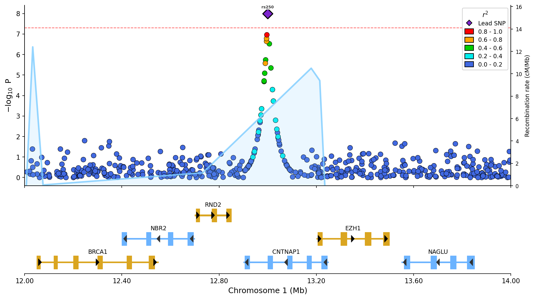
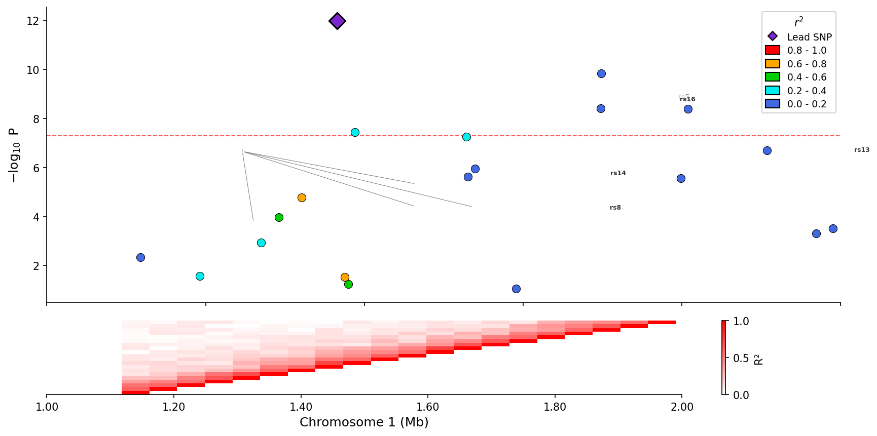
Regional association plot:
- Multi-species support: Built-in reference data for Canis lupus familiaris (CanFam3.1/CanFam4) and Felis catus (FelCat9), or optionally provide your own for any species
- LD coloring: SNPs colored by linkage disequilibrium (R²) with lead variant
- Gene tracks: Annotated gene/exon positions below the association plot
- Recombination rate: Overlay across region (Canis lupus familiaris built-in, or user-provided)
- SNP labels (matplotlib): Automatic labeling of top SNPs by p-value (RS IDs)
- Hover tooltips (Plotly and Bokeh): Detailed SNP data on hover
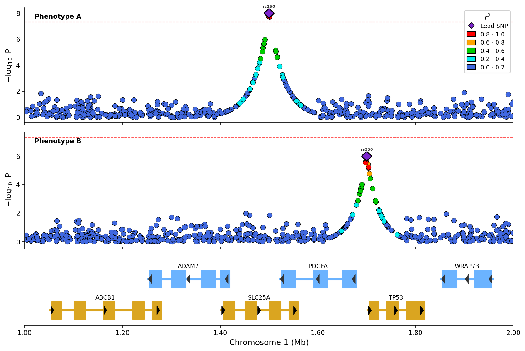
- Stacked plots: Compare multiple GWAS/phenotypes vertically
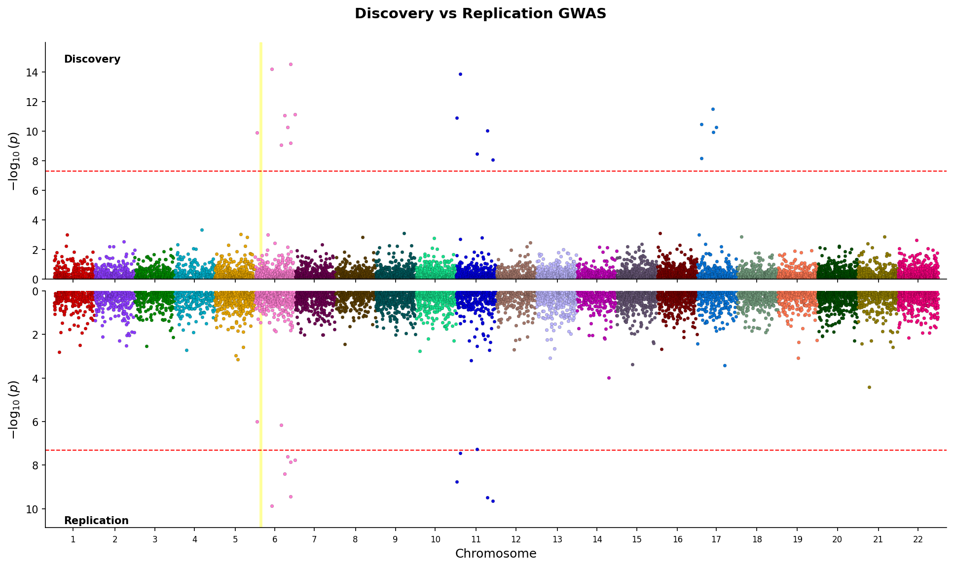
- Miami plots: Mirrored Manhattan plots for comparing two GWAS datasets (discovery vs replication)
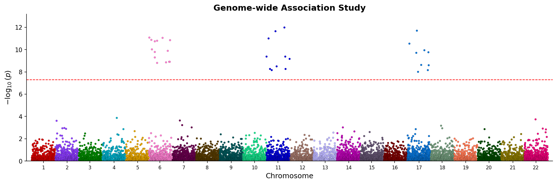
- Manhattan plots: Genome-wide association visualization with chromosome coloring
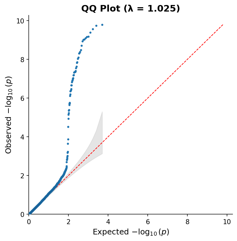
- QQ plots: Quantile-quantile plots with confidence bands and genomic inflation factor
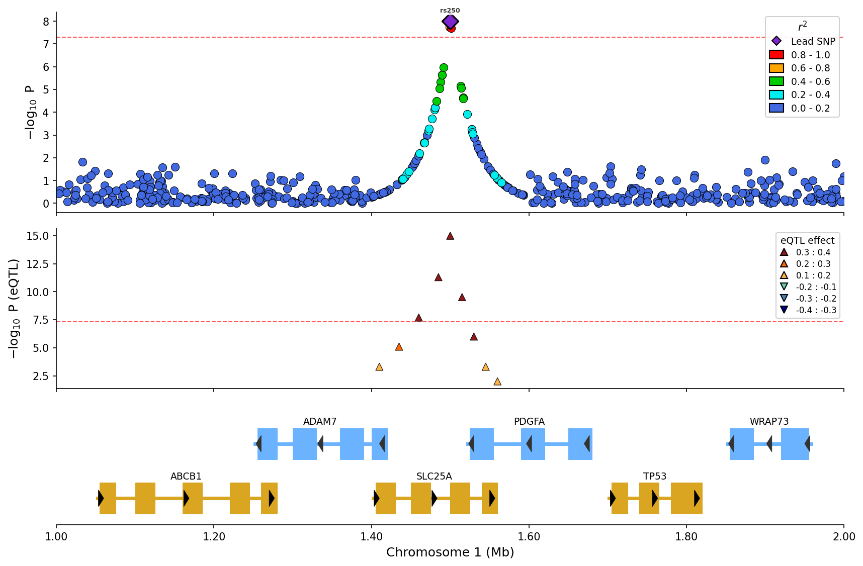
- eQTL plot: Expression QTL data aligned with association plots and gene tracks
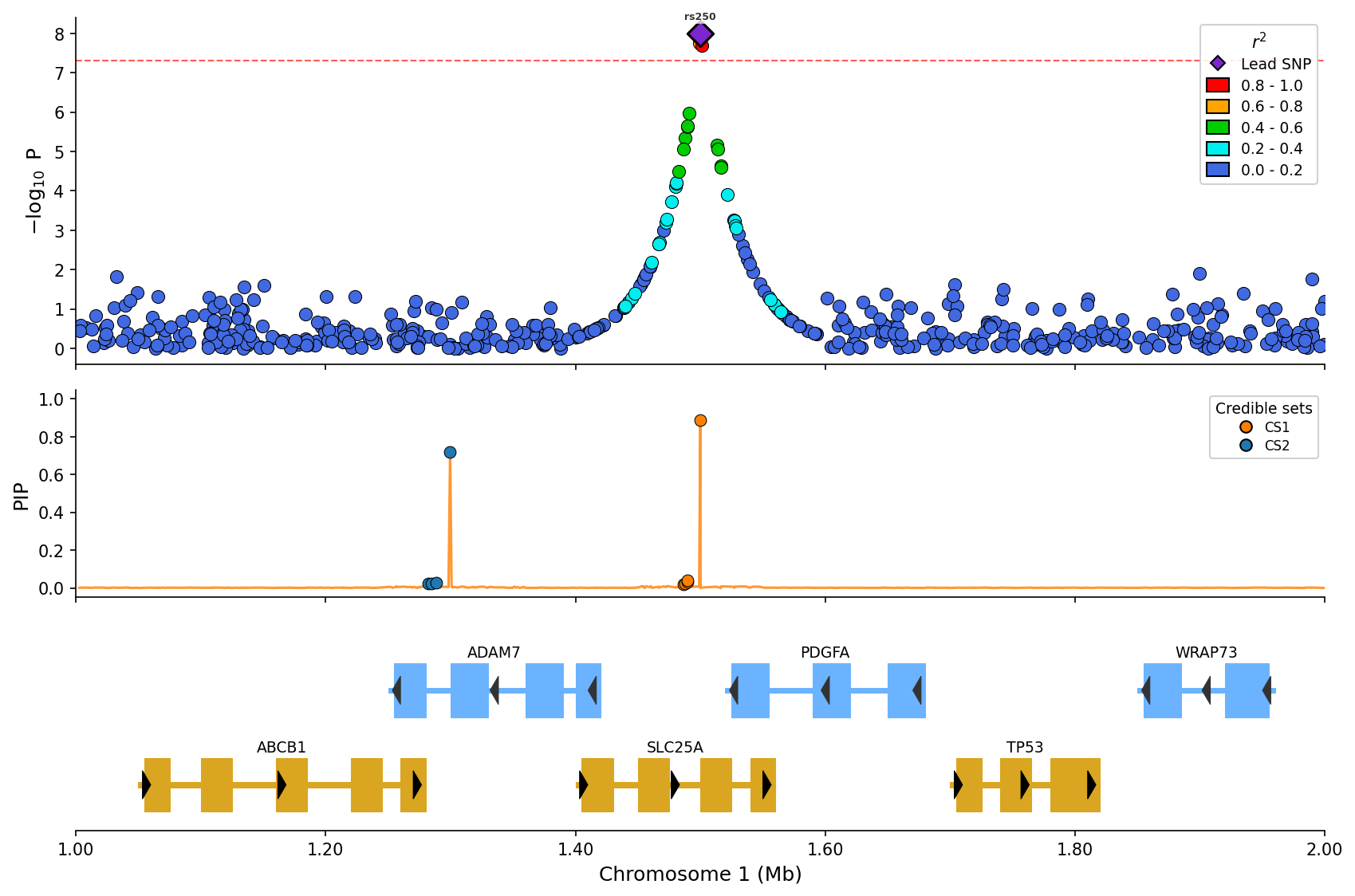
- Fine-mapping plots: Visualize SuSiE credible sets with posterior inclusion probabilities
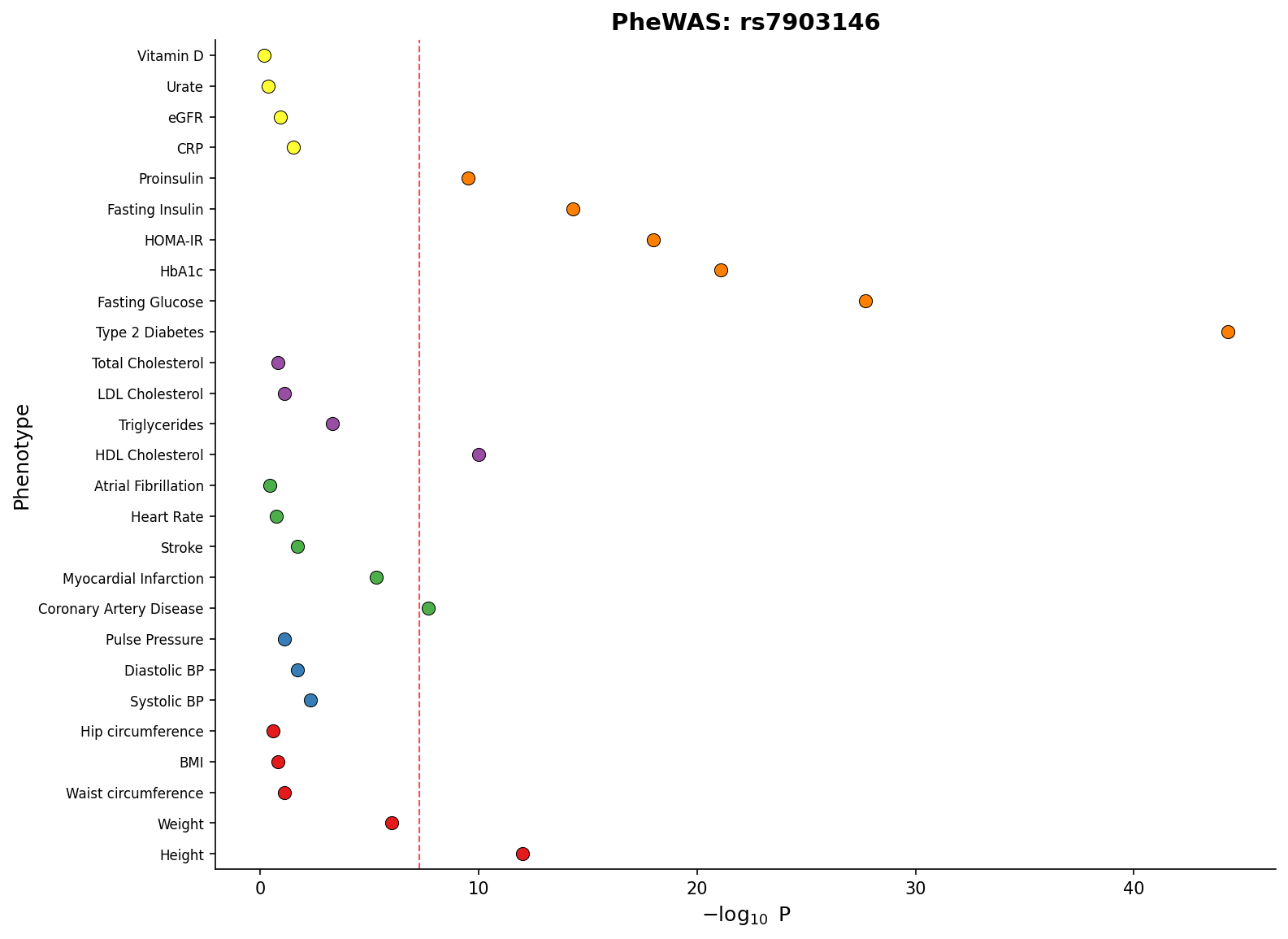
- PheWAS plots: Phenome-wide association study visualization across multiple phenotypes
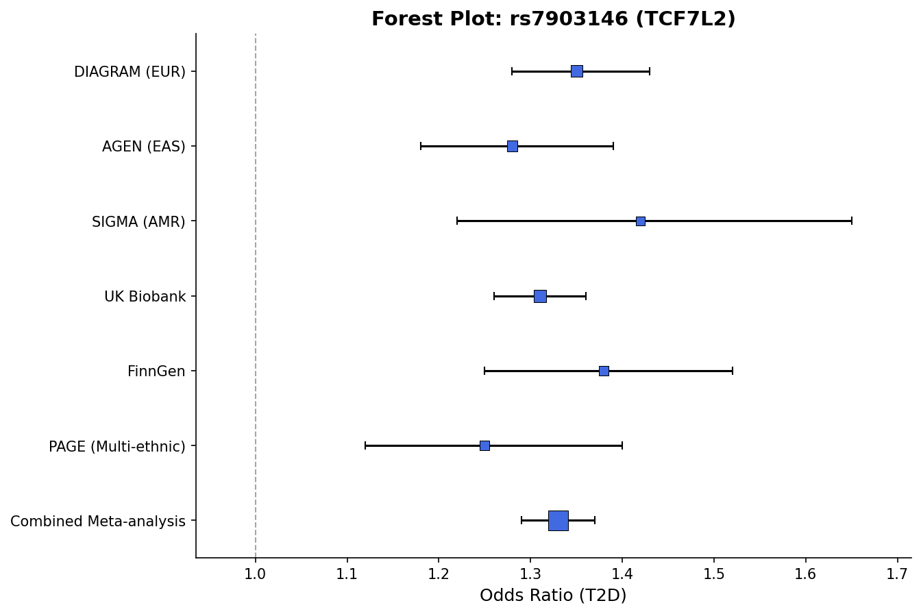
- Forest plots: Meta-analysis effect size visualization with confidence intervals
- LD heatmaps: Triangular heatmaps showing pairwise LD patterns, standalone or integrated below regional plots
- Colocalization plots: GWAS-eQTL scatter plots with LD coloring, correlation statistics, and effect direction visualization
- Multiple backends: matplotlib (publication-ready), plotly (interactive), bokeh (dashboard integration)
- Pandas and PySpark support: Works with both Pandas and PySpark DataFrames for large-scale genomics data
- Convenience data file loaders: Load and validate common GWAS, eQTL and fine-mapping file formats
- Automatic gene annotations: Fetch gene/exon data from Ensembl REST API with caching (human, mouse, rat, canine, feline, and any Ensembl species)
Installation
pip install pylocuszoom
Or with uv:
uv add pylocuszoom
Or with conda (Bioconda):
conda install -c bioconda pylocuszoom
Quick Start
from pylocuszoom import LocusZoomPlotter

# Initialize plotter (loads reference data for canine)
plotter = LocusZoomPlotter(species="canine", auto_genes=True)

# Plot with parameters passed directly
fig = plotter.plot(
    gwas_df,                        # DataFrame with pos, p_value, rs columns
    chrom=1,
    start=1000000,
    end=2000000,
    lead_pos=1500000,               # Highlight lead SNP
    show_recombination=True,        # Overlay recombination rate
)
fig.savefig("regional_plot.png", dpi=150)
Full Example
from pylocuszoom import LocusZoomPlotter

plotter = LocusZoomPlotter(
    species="canine",                   # or "feline", or None for custom
    plink_path="/path/to/plink",        # Optional, auto-detects if on PATH
)

fig = plotter.plot(
    gwas_df,
    chrom=1,
    start=1000000,
    end=2000000,
    lead_pos=1500000,
    ld_reference_file="genotypes",      # PLINK fileset (without extension)
    show_recombination=True,            # Overlay recombination rate
    snp_labels=True,                    # Label top SNPs
    label_top_n=5,                      # How many to label
    pos_col="ps",                       # Column name for position
    p_col="p_wald",                     # Column name for p-value
    rs_col="rs",                        # Column name for SNP ID
    figsize=(12, 8),
    genes_df=genes_df,                  # Gene annotations
    exons_df=exons_df,                  # Exon annotations
)
Genome Builds
The default genome build for canine is CanFam3.1. For CanFam4 data:
plotter = LocusZoomPlotter(species="canine", genome_build="canfam4")
Recombination maps are automatically lifted over from CanFam3.1 to CanFam4 coordinates using the UCSC liftOver chain file.
Using with Other Species
from pylocuszoom import LocusZoomPlotter

# Feline (LD and gene tracks, user provides recombination data)
plotter = LocusZoomPlotter(species="feline")

# Custom species (provide all reference data)
plotter = LocusZoomPlotter(
    species=None,
    recomb_data_dir="/path/to/recomb_maps/",
)

# Provide data per-plot
fig = plotter.plot(
    gwas_df,
    chrom=1,
    start=1000000,
    end=2000000,
    recomb_df=my_recomb_dataframe,
    genes_df=my_genes_df,
)
Automatic Gene Annotations
pyLocusZoom can automatically fetch gene annotations from Ensembl for any species:
from pylocuszoom import LocusZoomPlotter

# Enable automatic gene fetching
plotter = LocusZoomPlotter(species="human", auto_genes=True)

# No need to provide genes_df - fetched automatically
fig = plotter.plot(gwas_df, chrom=13, start=32000000, end=33000000)
Supported species aliases: human, mouse, rat, canine/dog, feline/cat, or any Ensembl species name.
Data is cached locally for fast subsequent plots. Maximum region size is 5Mb (Ensembl API limit).
Backends
pyLocusZoom supports multiple rendering backends (set at initialization):
from pylocuszoom import LocusZoomPlotter

# Static publication-quality plot (default)
plotter = LocusZoomPlotter(species="canine", backend="matplotlib")
fig = plotter.plot(gwas_df, chrom=1, start=1000000, end=2000000)
fig.savefig("plot.png", dpi=150)

# Interactive Plotly (hover tooltips, pan/zoom)
plotter = LocusZoomPlotter(species="canine", backend="plotly")
fig = plotter.plot(gwas_df, chrom=1, start=1000000, end=2000000)
fig.write_html("plot.html")

# Interactive Bokeh (dashboard-ready)
plotter = LocusZoomPlotter(species="canine", backend="bokeh")
fig = plotter.plot(gwas_df, chrom=1, start=1000000, end=2000000)
| Backend | Output | Best For | Features |
|---|---|---|---|
matplotlib |
Static PNG/PDF/SVG | Publication-ready figures | Full feature set with SNP labels |
plotly |
Interactive HTML | Web reports, exploration | Hover tooltips, pan/zoom |
bokeh |
Interactive HTML | Dashboard integration | Hover tooltips, pan/zoom |
Note: All backends support scatter plots, gene tracks, recombination overlay, and LD legend. SNP labels (auto-positioned with adjustText) are matplotlib-only; interactive backends use hover tooltips instead.
Stacked Plots
Compare multiple GWAS results vertically with shared x-axis:
from pylocuszoom import LocusZoomPlotter

plotter = LocusZoomPlotter(species="canine")

fig = plotter.plot_stacked(
    [gwas_height, gwas_bmi, gwas_whr],
    chrom=1,
    start=1000000,
    end=2000000,
    panel_labels=["Height", "BMI", "WHR"],
    genes_df=genes_df,
)
eQTL Overlay
Add expression QTL data as a separate panel:
from pylocuszoom import LocusZoomPlotter

eqtl_df = pd.DataFrame({
    "pos": [1000500, 1001200, 1002000],
    "p_value": [1e-6, 1e-4, 0.01],
    "gene": ["BRCA1", "BRCA1", "BRCA1"],
})

plotter = LocusZoomPlotter(species="canine")

fig = plotter.plot_stacked(
    [gwas_df],
    chrom=1,
    start=1000000,
    end=2000000,
    eqtl_df=eqtl_df,
    eqtl_gene="BRCA1",
    genes_df=genes_df,
)
Fine-mapping Visualization
Visualize SuSiE or other fine-mapping results with credible set coloring:
from pylocuszoom import LocusZoomPlotter

finemapping_df = pd.DataFrame({
    "pos": [1000500, 1001200, 1002000, 1003500],
    "pip": [0.85, 0.12, 0.02, 0.45],  # Posterior inclusion probability
    "cs": [1, 1, 0, 2],               # Credible set assignment (0 = not in CS)
})

plotter = LocusZoomPlotter(species="canine")

fig = plotter.plot_stacked(
    [gwas_df],
    chrom=1,
    start=1000000,
    end=2000000,
    finemapping_df=finemapping_df,
    finemapping_cs_col="cs",
    genes_df=genes_df,
)
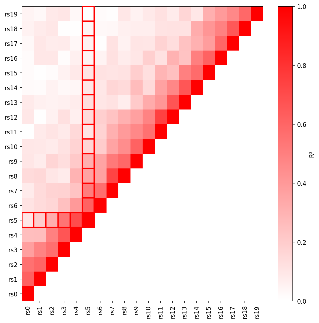
LD Heatmaps
Create triangular LD heatmaps showing pairwise linkage disequilibrium patterns:
from pylocuszoom import LDHeatmapPlotter

# ld_matrix is a square DataFrame with SNP IDs as index/columns
# snp_ids is a list of SNP IDs in the matrix

ld_plotter = LDHeatmapPlotter()
fig = ld_plotter.plot(
    ld_matrix,
    snp_ids,
    highlight_snp_id="rs12345",  # Highlight lead SNP
    metric="r2",                  # or "dprime"
)
fig.savefig("ld_heatmap.png", dpi=150)
Integrated LD Heatmap with Regional Plot
Add an LD heatmap panel below a regional association plot:
from pylocuszoom import LocusZoomPlotter

plotter = LocusZoomPlotter(species="canine")

fig = plotter.plot(
    gwas_df,
    chrom=1,
    start=1000000,
    end=2000000,
    lead_pos=1500000,
    ld_heatmap_df=ld_matrix,         # Pairwise LD matrix
    ld_heatmap_snp_ids=snp_ids,      # SNP IDs in matrix
    ld_heatmap_height=0.25,          # Panel height ratio
)
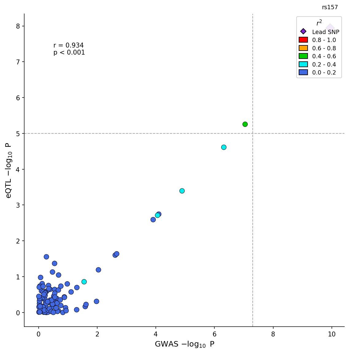
Colocalization Plots
Visualize GWAS-eQTL colocalization by comparing association signals in a scatter plot with LD coloring:
from pylocuszoom import ColocPlotter

# GWAS and eQTL data with matching positions
gwas_df = pd.DataFrame({
    "pos": positions,
    "p": gwas_pvalues,
    "ld_r2": ld_values,  # Optional: LD with lead SNP
})

eqtl_df = pd.DataFrame({
    "pos": positions,
    "p": eqtl_pvalues,
})

plotter = ColocPlotter()
fig = plotter.plot_coloc(
    gwas_df=gwas_df,
    eqtl_df=eqtl_df,
    pos_col="pos",
    gwas_p_col="p",
    eqtl_p_col="p",
    ld_col="ld_r2",
    gwas_threshold=5e-8,
    eqtl_threshold=1e-5,
)
fig.savefig("colocalization.png", dpi=150)
Advanced options include effect direction coloring and H4 posterior probability display:
fig = plotter.plot_coloc(
    gwas_df=gwas_df,
    eqtl_df=eqtl_df,
    pos_col="pos",
    gwas_p_col="p",
    eqtl_p_col="p",
    gwas_effect_col="beta",
    eqtl_effect_col="slope",
    color_by_effect=True,  # Green=congruent, Red=incongruent
    h4_posterior=0.85,     # Display coloc H4 probability
)
PheWAS Plots
Visualize associations of a single variant across multiple phenotypes:
from pylocuszoom import StatsPlotter

phewas_df = pd.DataFrame({
    "phenotype": ["Height", "BMI", "T2D", "CAD", "HDL"],
    "p_value": [1e-15, 0.05, 1e-8, 1e-3, 1e-10],
    "category": ["Anthropometric", "Anthropometric", "Metabolic", "Cardiovascular", "Lipids"],
})

stats_plotter = StatsPlotter()
fig = stats_plotter.plot_phewas(
    phewas_df,
    variant_id="rs12345",
    category_col="category",
)
Forest Plots
Create forest plots for meta-analysis visualization:
from pylocuszoom import StatsPlotter

forest_df = pd.DataFrame({
    "study": ["Study A", "Study B", "Study C", "Meta-analysis"],
    "effect": [0.45, 0.52, 0.38, 0.46],
    "ci_lower": [0.30, 0.35, 0.20, 0.40],
    "ci_upper": [0.60, 0.69, 0.56, 0.52],
    "weight": [25, 35, 20, 100],
})

stats_plotter = StatsPlotter()
fig = stats_plotter.plot_forest(
    forest_df,
    variant_id="rs12345",
    weight_col="weight",
)
Miami Plots
Compare two GWAS datasets with mirrored Manhattan plots (top panel ascending, bottom panel inverted):
from pylocuszoom import MiamiPlotter

plotter = MiamiPlotter(species="human")

fig = plotter.plot_miami(
    discovery_df,
    replication_df,
    chrom_col="chrom",
    pos_col="pos",
    p_col="p",
    top_label="Discovery",
    bottom_label="Replication",
    top_threshold=5e-8,
    bottom_threshold=1e-6,
    highlight_regions=[("6", 30_000_000, 35_000_000)],  # Highlight MHC region
)
fig.savefig("miami.png", dpi=150)
Interactive backends (Plotly/Bokeh) provide hover tooltips showing SNP details:
# Plotly - interactive HTML with hover tooltips
plotter = MiamiPlotter(species="human", backend="plotly")
fig = plotter.plot_miami(discovery_df, replication_df, ...)
fig.write_html("miami_interactive.html")

# Bokeh - dashboard-ready interactive plots
from bokeh.io import output_file, save
plotter = MiamiPlotter(species="human", backend="bokeh")
fig = plotter.plot_miami(discovery_df, replication_df, ...)
output_file("miami_bokeh.html")
save(fig)
Manhattan Plots
Create genome-wide Manhattan plots showing associations across all chromosomes:
from pylocuszoom import ManhattanPlotter

plotter = ManhattanPlotter(species="human")

fig = plotter.plot_manhattan(
    gwas_df,
    chrom_col="chrom",
    pos_col="pos",
    p_col="p",
    significance_threshold=5e-8,  # Genome-wide significance line
    figsize=(12, 5),
)
fig.savefig("manhattan.png", dpi=150)
Categorical Manhattan plots (PheWAS-style) are also supported:
fig = plotter.plot_manhattan(
    phewas_df,
    category_col="phenotype_category",
    p_col="pvalue",
)
QQ Plots
Create quantile-quantile plots to assess p-value distribution:
from pylocuszoom import ManhattanPlotter

plotter = ManhattanPlotter()

fig = plotter.plot_qq(
    gwas_df,
    p_col="p",
    show_confidence_band=True,  # 95% confidence band
    show_lambda=True,           # Genomic inflation factor in title
    figsize=(6, 6),
)
fig.savefig("qq_plot.png", dpi=150)
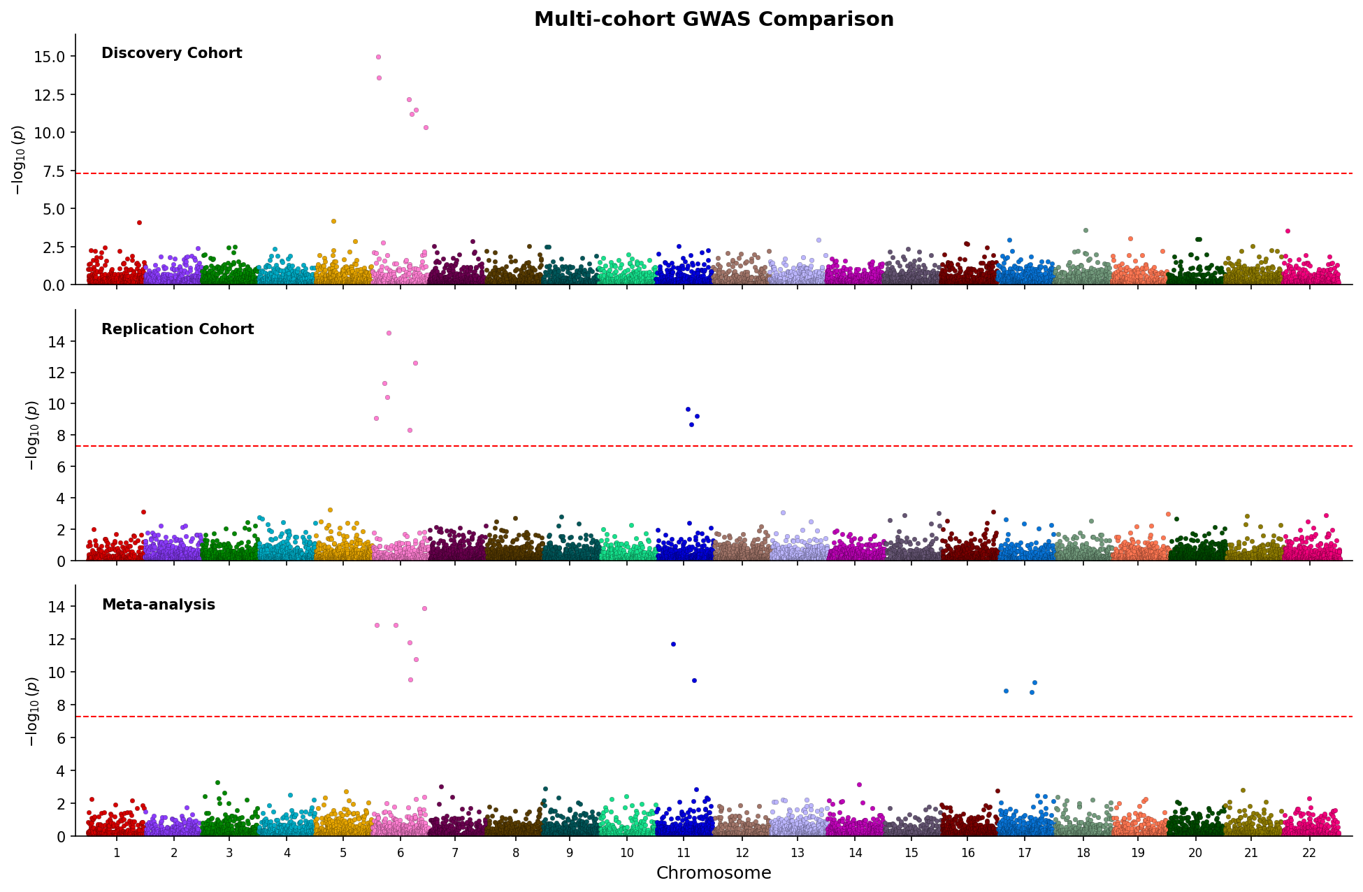
Stacked Manhattan Plots
Compare multiple GWAS results in vertically stacked Manhattan plots:
from pylocuszoom import ManhattanPlotter

plotter = ManhattanPlotter()

fig = plotter.plot_manhattan_stacked(
    [gwas_study1, gwas_study2, gwas_study3],
    chrom_col="chrom",
    pos_col="pos",
    p_col="p",
    panel_labels=["Study 1", "Study 2", "Study 3"],
    significance_threshold=5e-8,
    figsize=(12, 8),
    title="Multi-study GWAS Comparison",
)
fig.savefig("manhattan_stacked.png", dpi=150)
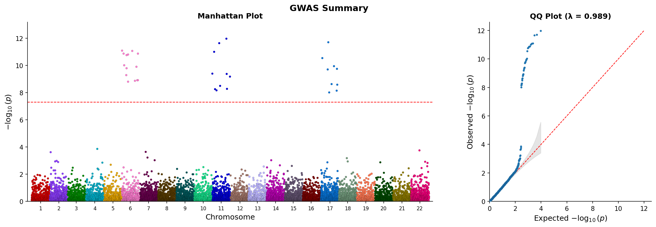
Manhattan and QQ Side-by-Side
Create combined Manhattan and QQ plots in a single figure:
from pylocuszoom import ManhattanPlotter

plotter = ManhattanPlotter()

fig = plotter.plot_manhattan_qq(
    gwas_df,
    chrom_col="chrom",
    pos_col="pos",
    p_col="p",
    significance_threshold=5e-8,
    show_confidence_band=True,
    show_lambda=True,
    figsize=(14, 5),
    title="GWAS Results",
)
fig.savefig("manhattan_qq.png", dpi=150)
PySpark Support
For large-scale genomics data, convert PySpark DataFrames with to_pandas() before plotting:
from pylocuszoom import LocusZoomPlotter, to_pandas

# Convert PySpark DataFrame (optionally sampled for very large data)
pandas_df = to_pandas(spark_gwas_df, sample_size=100000)
fig = plotter.plot(pandas_df, chrom=1, start=1000000, end=2000000)
Install PySpark support: uv add pylocuszoom[spark]
Loading Data from Files
pyLocusZoom includes loaders for common GWAS, eQTL, and fine-mapping file formats:
from pylocuszoom import (
    # GWAS loaders
    load_gwas,           # Auto-detect format
    load_plink_assoc,    # PLINK .assoc, .assoc.linear, .qassoc
    load_regenie,        # REGENIE .regenie
    load_bolt_lmm,       # BOLT-LMM .stats
    load_gemma,          # GEMMA .assoc.txt
    load_saige,          # SAIGE output
    # eQTL loaders
    load_gtex_eqtl,      # GTEx significant pairs
    load_eqtl_catalogue, # eQTL Catalogue format
    # Fine-mapping loaders
    load_susie,          # SuSiE output
    load_finemap,        # FINEMAP .snp output
    # Gene annotations
    load_gtf,            # GTF/GFF3 files
    load_bed,            # BED files
)

# Auto-detect GWAS format from filename
gwas_df = load_gwas("results.assoc.linear")

# Or use specific loader
gwas_df = load_regenie("ukb_results.regenie")

# Load gene annotations
genes_df = load_gtf("genes.gtf", feature_type="gene")
exons_df = load_gtf("genes.gtf", feature_type="exon")

# Load eQTL data
eqtl_df = load_gtex_eqtl("GTEx.signif_pairs.txt.gz", gene="BRCA1")

# Load fine-mapping results
fm_df = load_susie("susie_output.tsv")
Data Formats
GWAS Results DataFrame
Required columns (names configurable via pos_col, p_col, rs_col):
| Column | Type | Required | Description |
|---|---|---|---|
ps |
int | Yes | Genomic position in base pairs (1-based). Must match coordinate system of genes/recombination data. |
p_wald |
float | Yes | Association p-value (0 < p ≤ 1). Values are -log10 transformed for plotting. |
rs |
str | No | SNP identifier (e.g., "rs12345" or "chr1:12345"). Used for labeling top SNPs if snp_labels=True. |
Example:
gwas_df = pd.DataFrame({
    "ps": [1000000, 1000500, 1001000],
    "p_wald": [1e-8, 1e-6, 0.05],
    "rs": ["rs123", "rs456", "rs789"],
})
Genes DataFrame
| Column | Type | Required | Description |
|---|---|---|---|
chr |
str or int | Yes | Chromosome identifier. Accepts "1", "chr1", or 1. The "chr" prefix is stripped for matching. |
start |
int | Yes | Gene start position (bp, 1-based). Transcript start for strand-aware genes. |
end |
int | Yes | Gene end position (bp, 1-based). Must be >= start. |
gene_name |
str | Yes | Gene symbol displayed in track (e.g., "BRCA1", "TP53"). Keep short for readability. |
Example:
genes_df = pd.DataFrame({
    "chr": ["1", "1", "1"],
    "start": [1000000, 1050000, 1100000],
    "end": [1020000, 1080000, 1150000],
    "gene_name": ["GENE1", "GENE2", "GENE3"],
})
Exons DataFrame (optional)
Provides exon/intron structure. If omitted, genes are drawn as simple rectangles.
| Column | Type | Required | Description |
|---|---|---|---|
chr |
str or int | Yes | Chromosome identifier. |
start |
int | Yes | Exon start position (bp). |
end |
int | Yes | Exon end position (bp). |
gene_name |
str | Yes | Parent gene symbol. Must match gene_name in genes DataFrame. |
Recombination DataFrame
| Column | Type | Required | Description |
|---|---|---|---|
pos |
int | Yes | Genomic position (bp). Should span the plotted region with reasonable density (every ~10kb). |
rate |
float | Yes | Recombination rate in centiMorgans per megabase (cM/Mb). Typical range: 0-50 cM/Mb. |
Example:
recomb_df = pd.DataFrame({
    "pos": [1000000, 1010000, 1020000],
    "rate": [0.5, 2.3, 1.1],
})
Recombination Map Files
When using recomb_data_dir, files must be named chr{N}_recomb.tsv (e.g., chr1_recomb.tsv, chrX_recomb.tsv).
Format: Tab-separated with header row:
| Column | Description |
|---|---|
chr |
Chromosome number (without "chr" prefix) |
pos |
Position in base pairs |
rate |
Recombination rate (cM/Mb) |
cM |
Cumulative genetic distance (optional, not used for plotting) |
chr	pos	rate	cM
1	10000	0.5	0.005
1	20000	1.2	0.017
1	30000	0.8	0.025
Reference Data
Canine recombination maps are downloaded from Campbell et al. 2016 on first use.
To manually download:
from pylocuszoom import download_canine_recombination_maps

download_canine_recombination_maps()
Logging
Logging uses loguru and is configured via the log_level parameter (default: "INFO"):
# Suppress logging
plotter = LocusZoomPlotter(log_level=None)

# Enable DEBUG level for troubleshooting
plotter = LocusZoomPlotter(log_level="DEBUG")
Requirements
- Python >= 3.10
- matplotlib >= 3.5.0
- pandas >= 1.4.0
- numpy >= 1.21.0
- loguru >= 0.7.0
- plotly >= 5.0.0
- bokeh >= 3.8.2
- kaleido >= 0.2.0 (for plotly static export)
- pyliftover >= 0.4 (for CanFam4 coordinate liftover)
- PLINK 1.9 (for LD calculations) - must be on PATH or specify
plink_path
Optional:
- pyspark >= 3.0.0 (for PySpark DataFrame support) -
uv add pylocuszoom[spark]
Documentation
- User Guide - Comprehensive documentation with API reference
- Code Map - Architecture diagram with source code links
- Architecture - Design decisions and component overview
- Example Notebook - Interactive tutorial
- CHANGELOG - Version history
License
GPL-3.0-or-later
Project details
Verified details
These details have been verified by PyPIProject links
GitHub Statistics
Maintainers
Release history Release notifications | RSS feed


Download files
Download the file for your platform. If you're not sure which to choose, learn more about installing packages.
Source Distribution
Built Distribution
Filter files by name, interpreter, ABI, and platform.
If you're not sure about the file name format, learn more about wheel file names.
Copy a direct link to the current filters
File details
Details for the file pylocuszoom-1.3.7.tar.gz.
File metadata
- Download URL: pylocuszoom-1.3.7.tar.gz
- Upload date:
- Size: 26.1 MB
- Tags: Source
- Uploaded using Trusted Publishing? Yes
- Uploaded via: twine/6.1.0 CPython/3.13.7
File hashes
| Algorithm | Hash digest | |
|---|---|---|
| SHA256 |
a8aec0ad19662cce98f99f21f1a5aac7362813a8de0273e167a1ff7fafbb4a63
|
|
| MD5 |
5ce50ac17557897acb35191cf6d07d9a
|
|
| BLAKE2b-256 |
56e1c570683772e6ddfe51bfd7d81df10da0ab368de6f52ceb967ca147b71e25
|
Provenance
The following attestation bundles were made for pylocuszoom-1.3.7.tar.gz:
Publisher:
publish.yml on michael-denyer/pyLocusZoom
-
Statement:
-
Statement type:
https://in-toto.io/Statement/v1 -
Predicate type:
https://docs.pypi.org/attestations/publish/v1 -
Subject name:
pylocuszoom-1.3.7.tar.gz -
Subject digest:
a8aec0ad19662cce98f99f21f1a5aac7362813a8de0273e167a1ff7fafbb4a63 - Sigstore transparency entry: 1113646759
- Sigstore integration time:
-
Permalink:
michael-denyer/pyLocusZoom@02ba8b9c3e8427c20d3f3ea4988b6bcbee6b1834 -
Branch / Tag:
refs/tags/v1.3.7 - Owner: https://github.com/michael-denyer
-
Access:
public
-
Token Issuer:
https://token.actions.githubusercontent.com -
Runner Environment:
github-hosted -
Publication workflow:
publish.yml@02ba8b9c3e8427c20d3f3ea4988b6bcbee6b1834 -
Trigger Event:
release
-
Statement type:
File details
Details for the file pylocuszoom-1.3.7-py3-none-any.whl.
File metadata
- Download URL: pylocuszoom-1.3.7-py3-none-any.whl
- Upload date:
- Size: 138.6 kB
- Tags: Python 3
- Uploaded using Trusted Publishing? Yes
- Uploaded via: twine/6.1.0 CPython/3.13.7
File hashes
| Algorithm | Hash digest | |
|---|---|---|
| SHA256 |
252fea513b6056aa661baea49c8ba98e1df6bf24bd11290fb1c534d9b89eebff
|
|
| MD5 |
28de45e14bd3a2c34a381e4bd9f3a504
|
|
| BLAKE2b-256 |
6a7e265735760dd1685a4c57a5505795e00fddb52a11408ec8956344c16be47a
|
Provenance
The following attestation bundles were made for pylocuszoom-1.3.7-py3-none-any.whl:
Publisher:
publish.yml on michael-denyer/pyLocusZoom
-
Statement:
-
Statement type:
https://in-toto.io/Statement/v1 -
Predicate type:
https://docs.pypi.org/attestations/publish/v1 -
Subject name:
pylocuszoom-1.3.7-py3-none-any.whl -
Subject digest:
252fea513b6056aa661baea49c8ba98e1df6bf24bd11290fb1c534d9b89eebff - Sigstore transparency entry: 1113646761
- Sigstore integration time:
-
Permalink:
michael-denyer/pyLocusZoom@02ba8b9c3e8427c20d3f3ea4988b6bcbee6b1834 -
Branch / Tag:
refs/tags/v1.3.7 - Owner: https://github.com/michael-denyer
-
Access:
public
-
Token Issuer:
https://token.actions.githubusercontent.com -
Runner Environment:
github-hosted -
Publication workflow:
publish.yml@02ba8b9c3e8427c20d3f3ea4988b6bcbee6b1834 -
Trigger Event:
release
-
Statement type:


