pyLocusZoom

Designed for publication-ready GWAS visualization with regional association plots, gene tracks, eQTL, PheWAS, fine-mapping, and forest plots.

Inspired by LocusZoom and locuszoomr.

Features

1. Regional association plot:

   • Multi-species support: Built-in reference data for Canis lupus familiaris (CanFam3.1/CanFam4) and Felis catus (FelCat9), or optionally provide your own for any species
   • LD coloring: SNPs colored by linkage disequilibrium (R²) with lead variant
   • Gene tracks: Annotated gene/exon positions below the association plot
   • Recombination rate: Overlay across region (Canis lupus familiaris built-in, or user-provided)
   • SNP labels (matplotlib): Automatic labeling of top SNPs by p-value (RS IDs)
   • Hover tooltips (Plotly and Bokeh): Detailed SNP data on hover

   Regional association plot with LD coloring, gene/exon track, recombination rate overlay (blue line), and top SNP labels.

2. Stacked plots: Compare multiple GWAS/phenotypes vertically

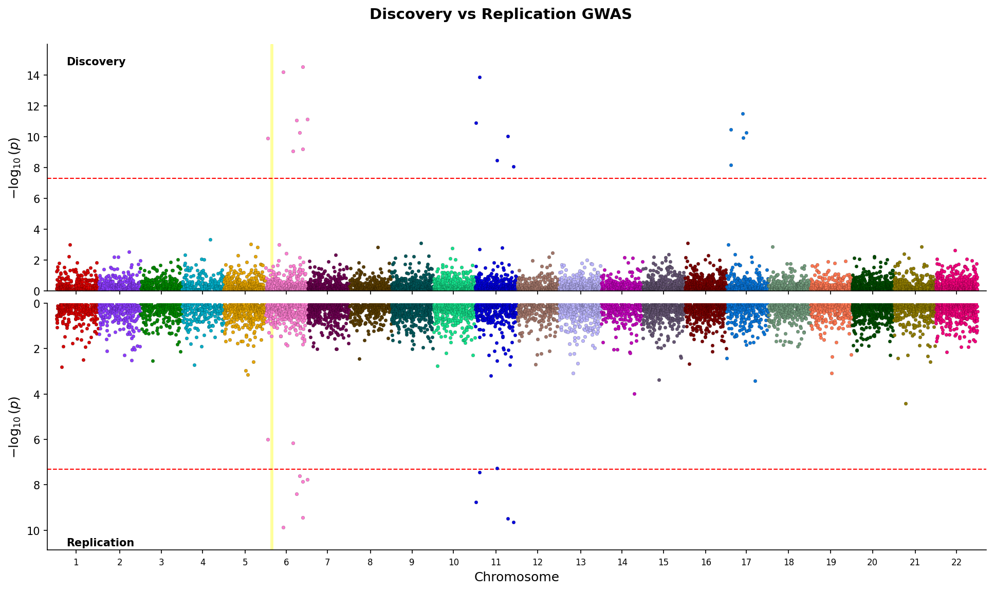
3. Miami plots: Mirrored Manhattan plots for comparing two GWAS datasets (discovery vs replication)

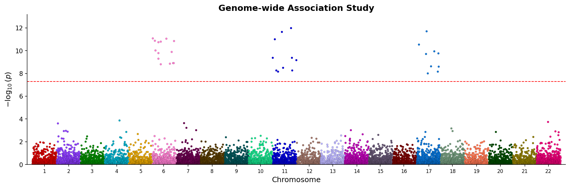
4. Manhattan plots: Genome-wide association visualization with chromosome coloring

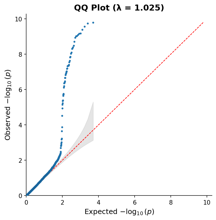
5. QQ plots: Quantile-quantile plots with confidence bands and genomic inflation factor

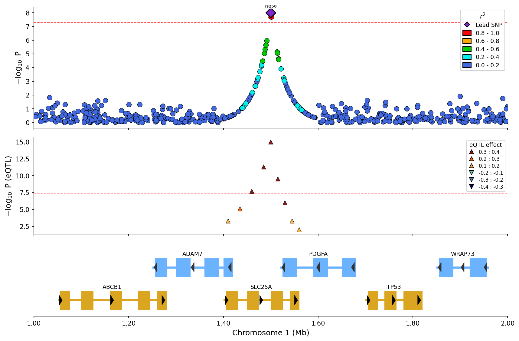
6. eQTL plot: Expression QTL data aligned with association plots and gene tracks

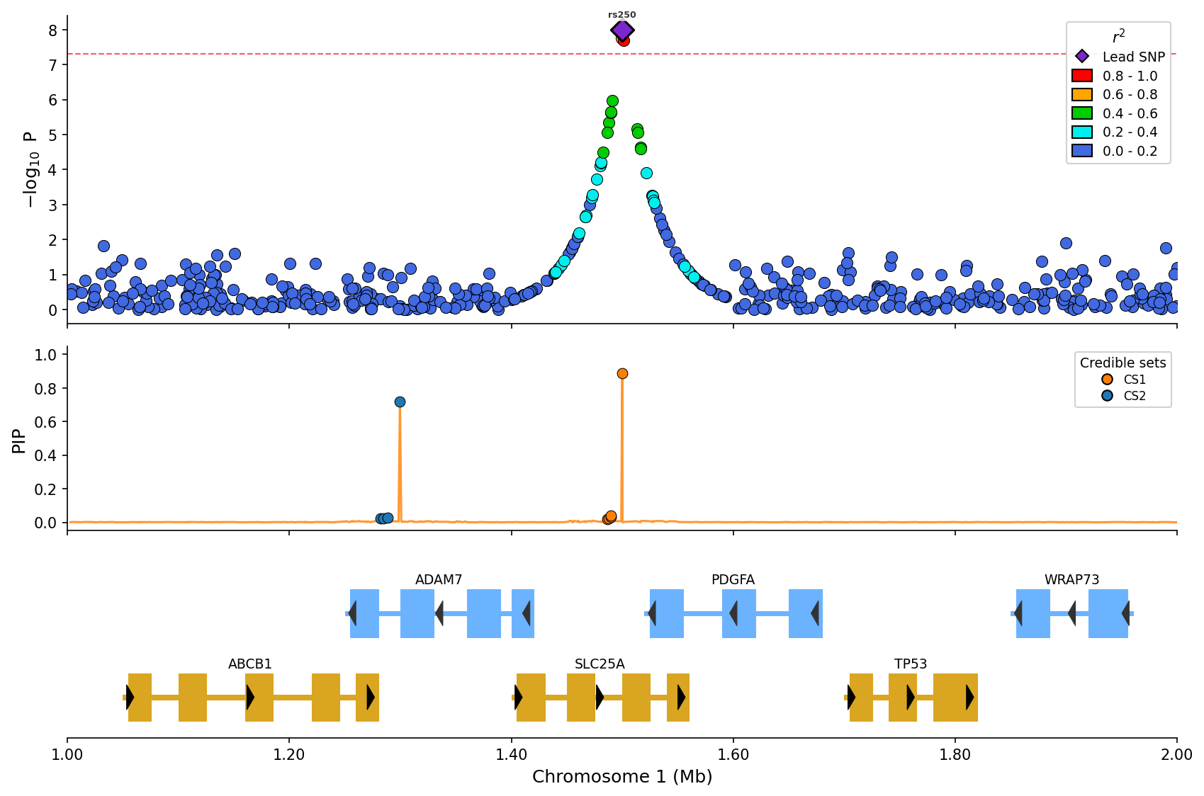
7. Fine-mapping plots: Visualize SuSiE credible sets with posterior inclusion probabilities

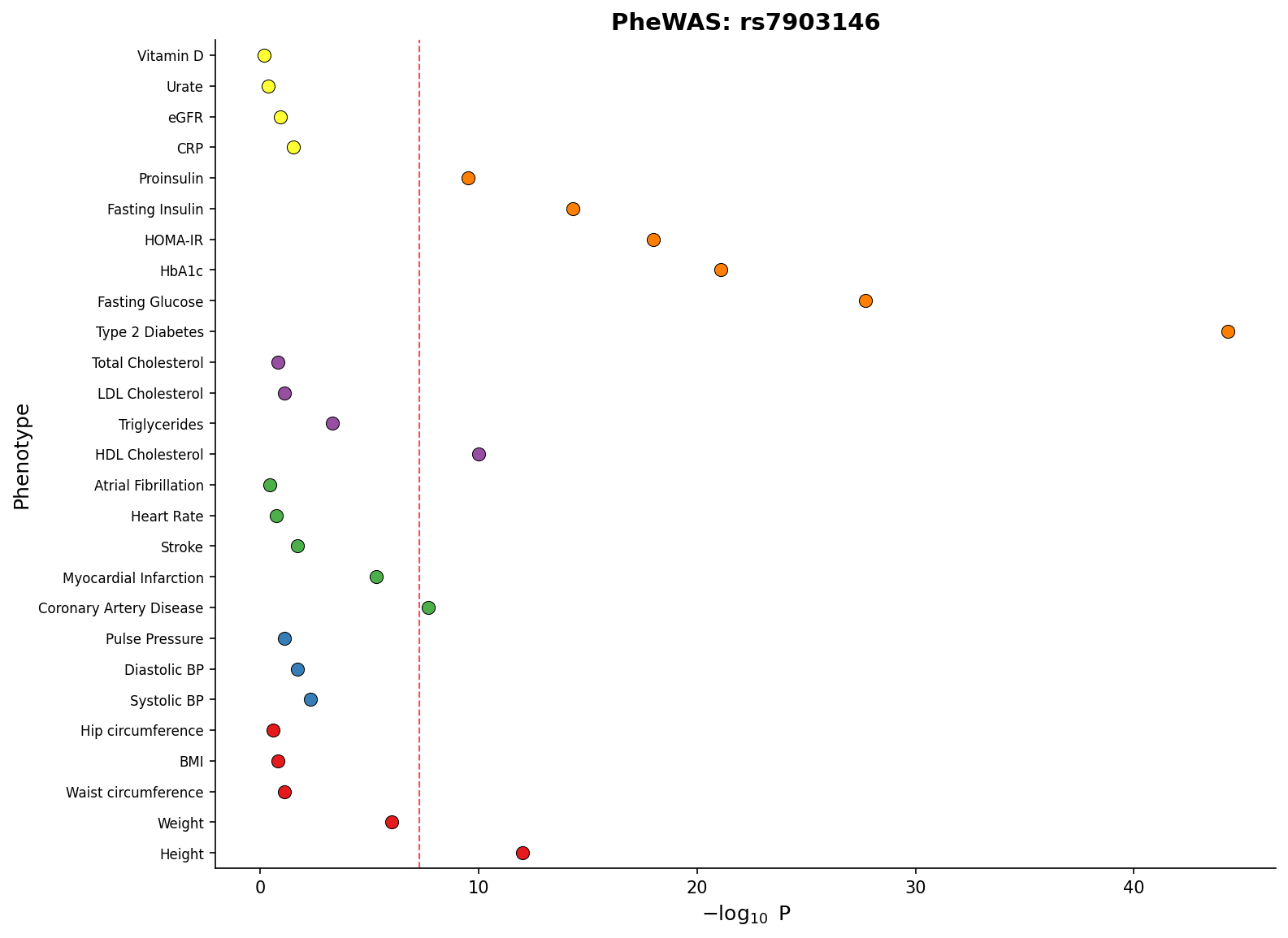
8. PheWAS plots: Phenome-wide association study visualization across multiple phenotypes

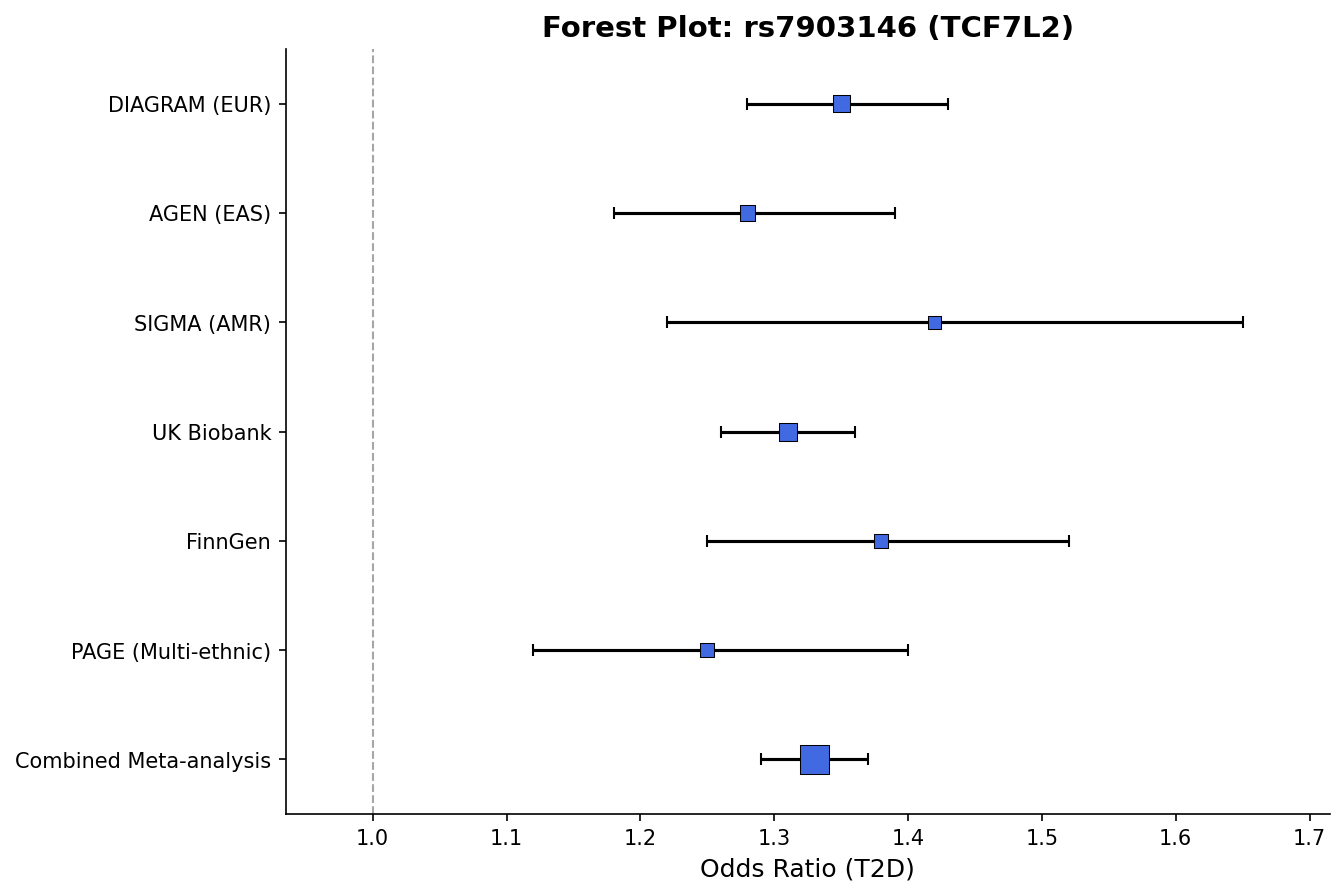
9. Forest plots: Meta-analysis effect size visualization with confidence intervals

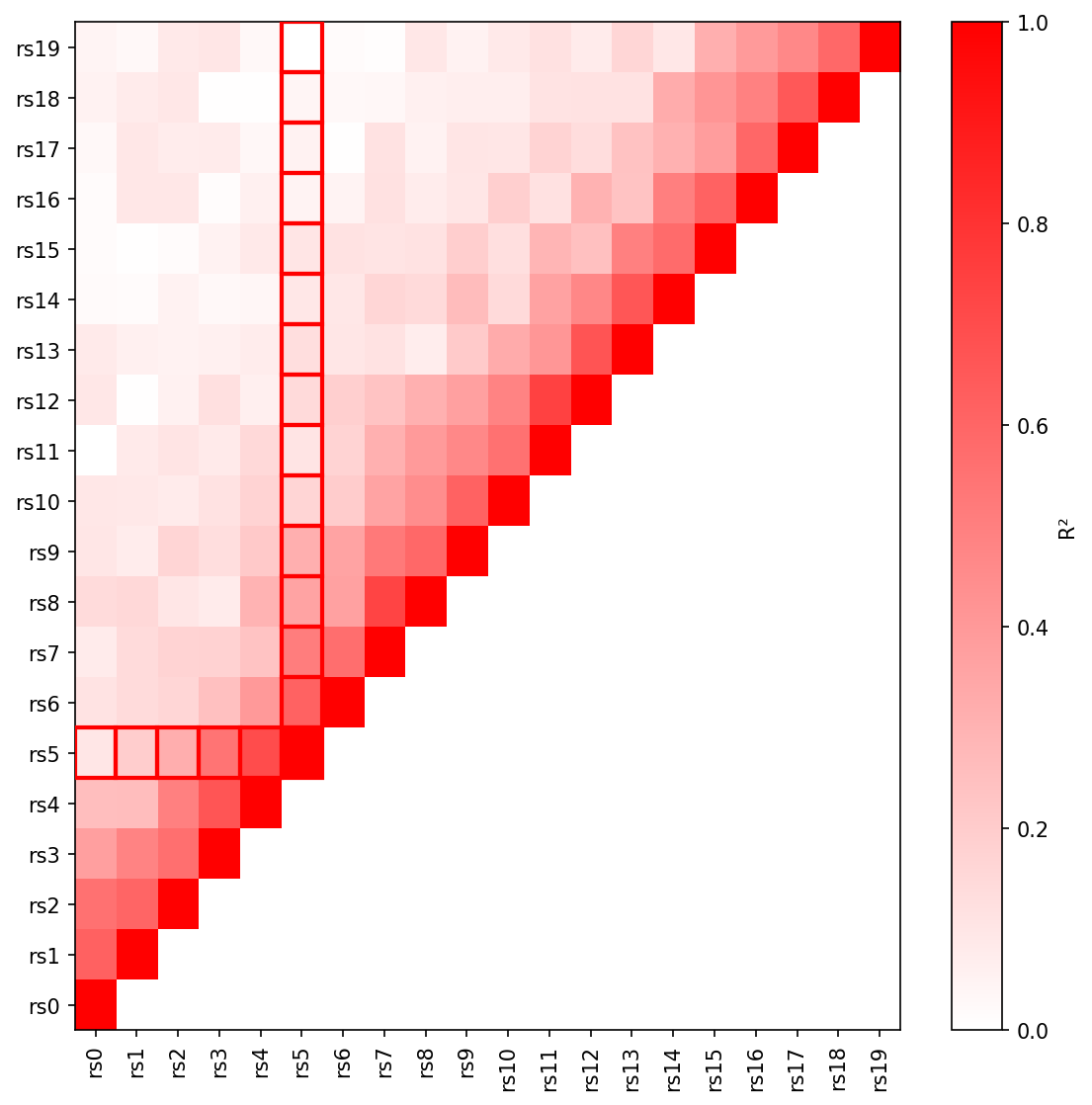
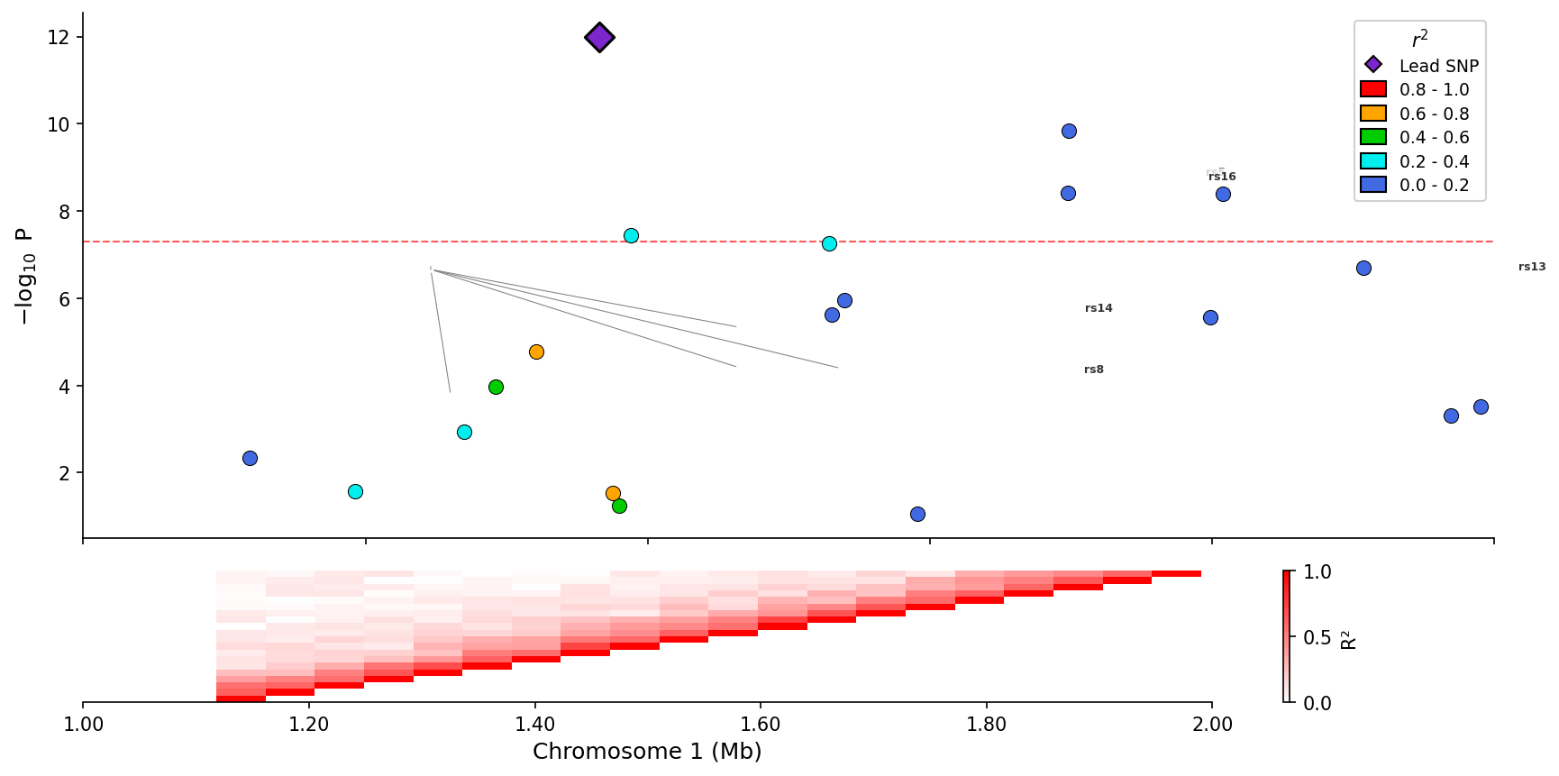
10. LD heatmaps: Triangular heatmaps showing pairwise LD patterns, standalone or integrated below regional plots

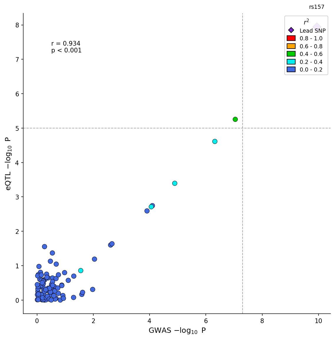
11. Colocalization plots: GWAS-eQTL scatter plots with LD coloring, correlation statistics, and effect direction visualization

12. Multiple backends: matplotlib (publication-ready), plotly (interactive), bokeh (dashboard integration)

13. Pandas and PySpark support: Works with both Pandas and PySpark DataFrames for large-scale genomics data

14. Convenience data file loaders: Load and validate common GWAS, eQTL and fine-mapping file formats

15. Automatic gene annotations: Fetch gene/exon data with caching, from UCSC for CanFam3.1, CanFam4 and FelCat9 and from the Ensembl REST API for human, mouse, rat and any other Ensembl species

Installation

pip install pylocuszoom

Or with uv:

uv add pylocuszoom

Or with conda (Bioconda):

conda install -c bioconda pylocuszoom

PySpark DataFrame support is an extra: pip install "pylocuszoom[spark]". LD colouring from a genotype fileset needs PLINK 1.9 on your PATH, or its location passed as plink_path.

Quick Start

from pylocuszoom import LDConfig, LocusZoomPlotter

# Initialize plotter (loads reference data for canine)
plotter = LocusZoomPlotter(species="canine", auto_genes=True)

# The region is passed directly; every other option lives on a config model
fig = plotter.plot(
    gwas_df,                        # DataFrame with chr, pos, p_value, rs columns
    chrom=1,
    start=1000000,
    end=2000000,
    ld=LDConfig(lead_pos=1500000),  # Highlight lead SNP
)
fig.savefig("regional_plot.png", dpi=150)

Pass backend="plotly" or backend="bokeh" to the plotter for an interactive figure with hover tooltips. The User Guide covers every plot type, the config models, the file loaders, the input column formats and species support.

Gallery

Each figure below links to the User Guide section with its code.

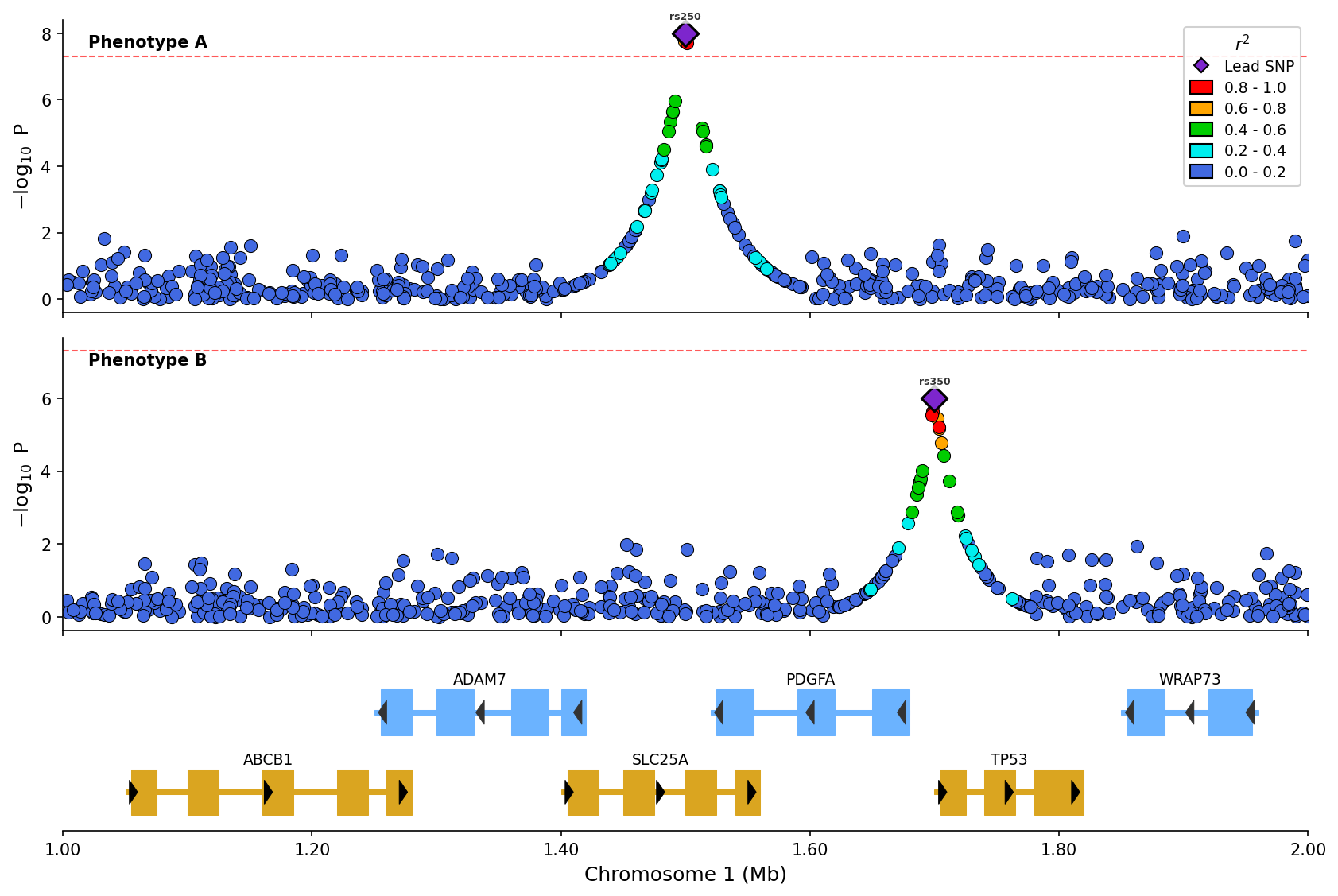
Stacked regional plots

Compare several GWAS over one region, with a shared gene track. User Guide

Stacked plot comparing two phenotypes with LD coloring and shared gene track.

eQTL overlay

Expression QTL results in their own panel below the association plot. User Guide

eQTL overlay with effect direction (up/down triangles) and magnitude binning.

Fine-mapping

SuSiE, FINEMAP, CAVIAR or PolyFun results, with credible sets coloured. User Guide

Fine-mapping visualization with PIP line and credible set coloring (CS1/CS2).

LD heatmaps

Triangular pairwise LD heatmaps, standalone or as a panel below a regional plot. User Guide

Triangular LD heatmap with R² values and lead SNP highlighted.

Regional association plot with integrated LD heatmap panel below.

Colocalization

GWAS against eQTL significance, coloured by LD or by effect-direction agreement. User Guide

GWAS-eQTL colocalization scatter plot with LD coloring and correlation statistics.

PheWAS

One variant's associations across phenotypes, grouped by category. User Guide

PheWAS plot showing associations across phenotype categories with significance threshold.

Forest plots

Effect sizes with confidence intervals across studies. User Guide

Forest plot with effect sizes, confidence intervals, and weight-proportional markers.

Miami plots

Two GWAS mirrored about a shared chromosome axis. User Guide

Miami plot comparing discovery and replication GWAS with mirrored y-axes and region highlighting.

Manhattan plots

Genome-wide associations by chromosome, or by category. User Guide

Manhattan plot showing genome-wide associations with chromosome coloring and significance threshold.

QQ plots

Observed against expected p-values, with a confidence band and λ. User Guide

QQ plot with 95% confidence band and genomic inflation factor (λ).

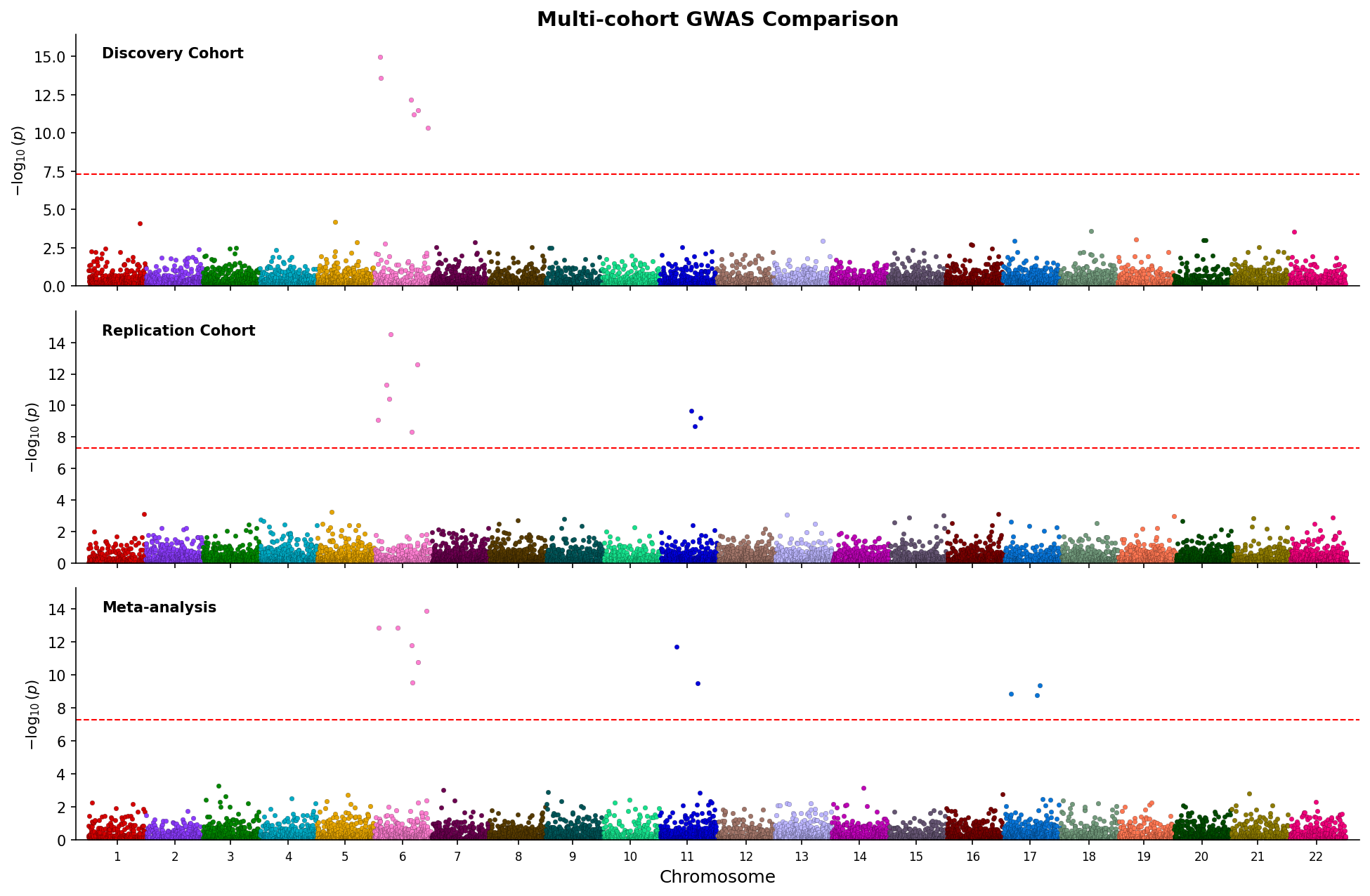
Stacked Manhattan plots

Several GWAS on one chromosome axis. User Guide

Stacked Manhattan plots comparing three GWAS studies with shared chromosome axis.

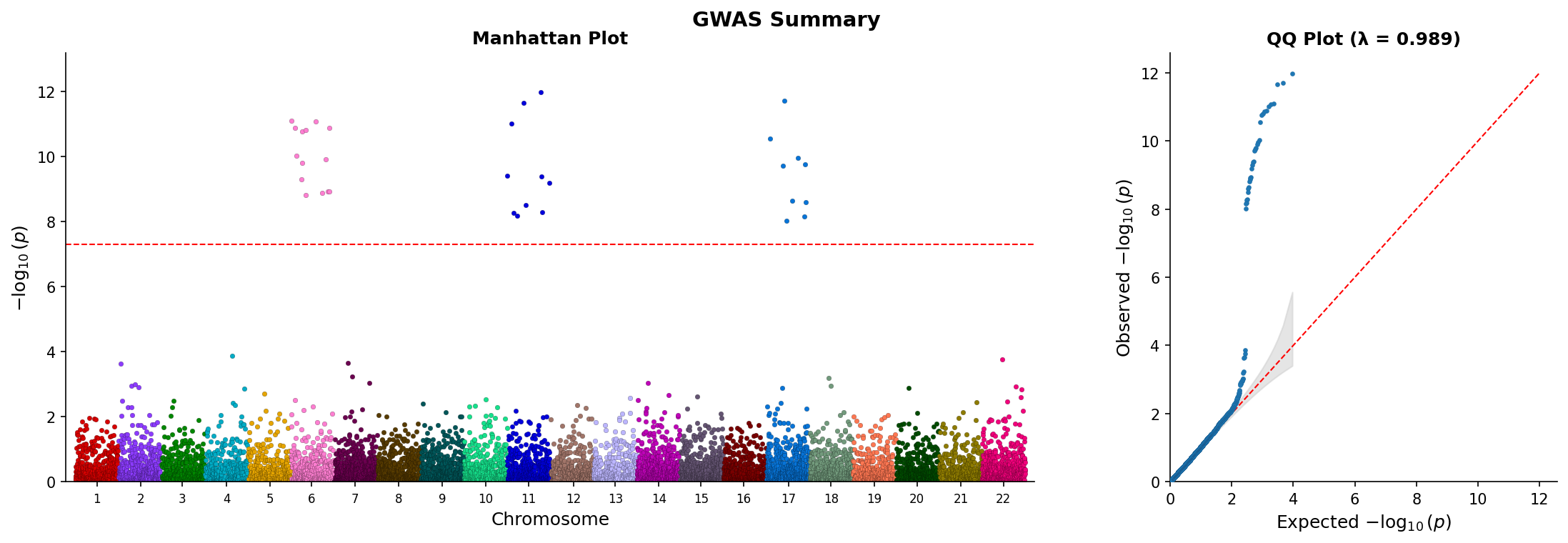
Manhattan and QQ side by side

A one-figure GWAS summary. Every genome-wide plot takes a GenomeWideStyle for palette, point and font styling. User Guide

Combined Manhattan and QQ plot showing genome-wide associations and p-value distribution.

Documentation

• Getting Started - Installation and first plot
• User Guide - Every plot type, the config models, loaders, data formats and species support
• Configuration - Cache locations and the environment variables that move them
• Architecture - Design decisions and component overview
• Code Map - Architecture diagram with source code links
• Development - Dev setup, pre-commit hooks, contributing workflow
• Testing - Running and writing tests
• Example Notebook - Interactive tutorial
• CHANGELOG - Version history

Citation

If you use pyLocusZoom in your research, please cite it. GitHub's "Cite this repository" button reads CITATION.cff, and each GitHub release is archived on Zenodo with its own DOI. The concept DOI 10.5281/zenodo.22665975 always resolves to the latest version.

@software{denyer_pylocuszoom,
  author  = {Denyer, Michael},
  title   = {pyLocusZoom: Python library for multi-species GWAS visualization},
  url     = {https://github.com/michael-denyer/pyLocusZoom},
  doi     = {10.5281/zenodo.22665975},
  license = {GPL-3.0-or-later}
}

License

GPL-3.0-or-later