









pyLocusZoom
Designed for publication-ready GWAS visualization with regional association plots, gene tracks, eQTL, PheWAS, fine-mapping, and forest plots.
Inspired by LocusZoom and locuszoomr.
Features
-
Regional association plot:
- Multi-species support: Built-in reference data for Canis lupus familiaris (CanFam3.1/CanFam4) and Felis catus (FelCat9), or optionally provide your own for any species
- LD coloring: SNPs colored by linkage disequilibrium (R²) with lead variant
- Gene tracks: Annotated gene/exon positions below the association plot
- Recombination rate: Overlay across region (Canis lupus familiaris built-in, or user-provided)
- SNP labels (matplotlib): Automatic labeling of top SNPs by p-value (RS IDs)
- Hover tooltips (Plotly and Bokeh): Detailed SNP data on hover
Regional association plot with LD coloring, gene/exon track, recombination rate overlay (blue line), and top SNP labels.
-
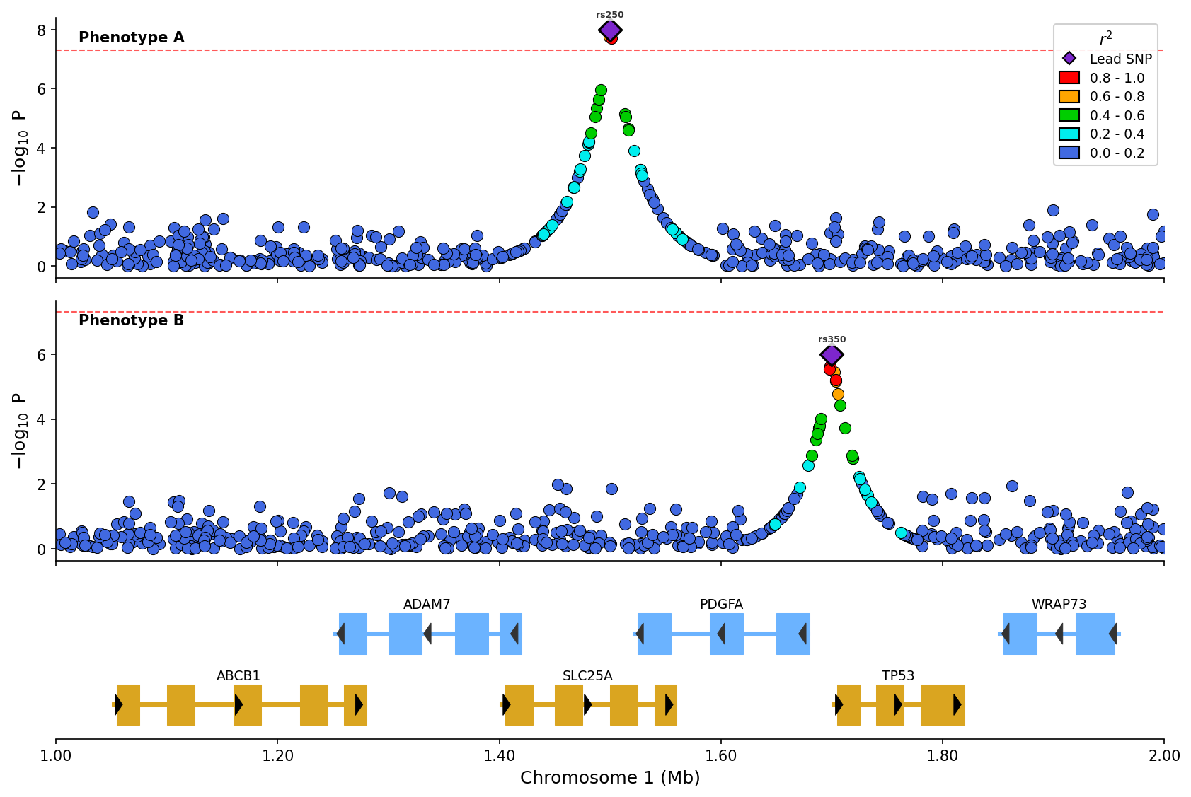
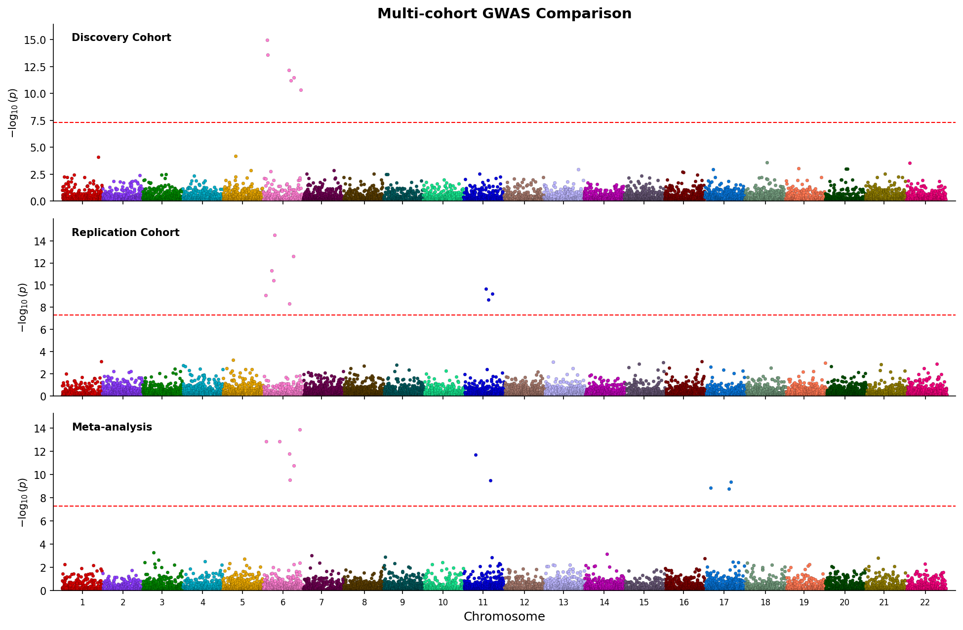
Stacked plots: Compare multiple GWAS/phenotypes vertically
-
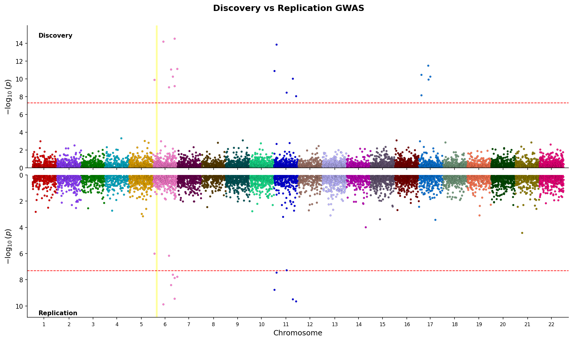
Miami plots: Mirrored Manhattan plots for comparing two GWAS datasets (discovery vs replication)
-
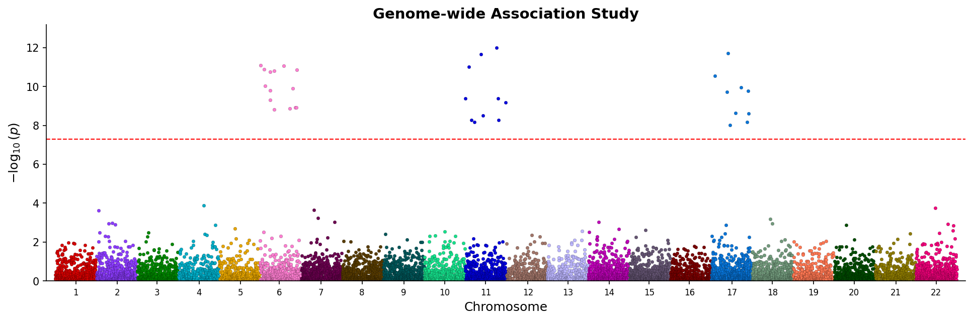
Manhattan plots: Genome-wide association visualization with chromosome coloring
-
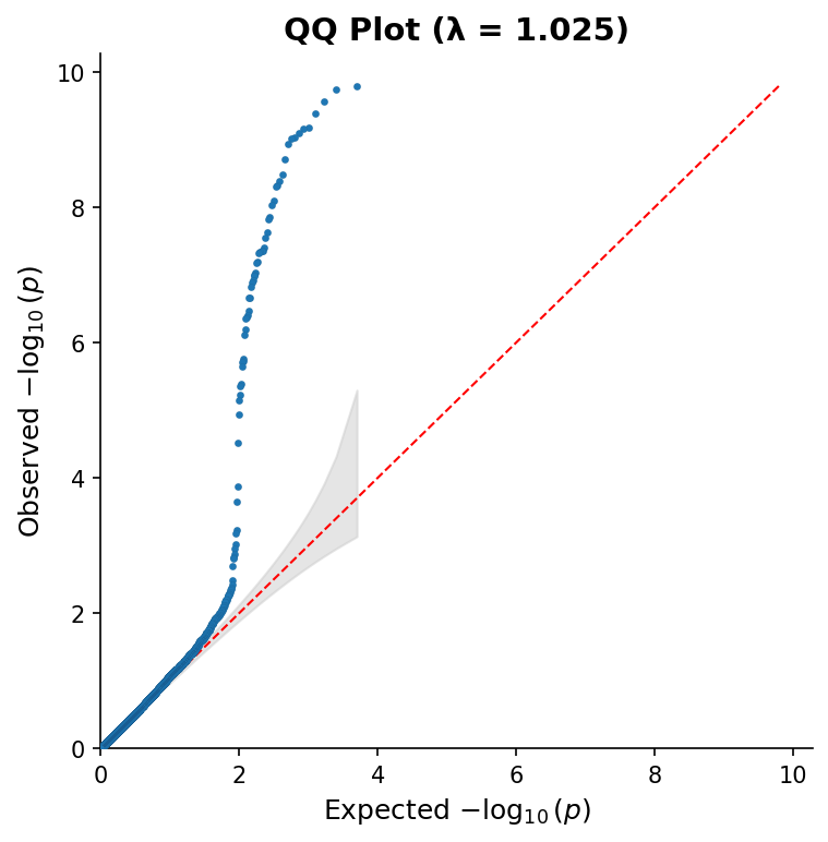
QQ plots: Quantile-quantile plots with confidence bands and genomic inflation factor
-
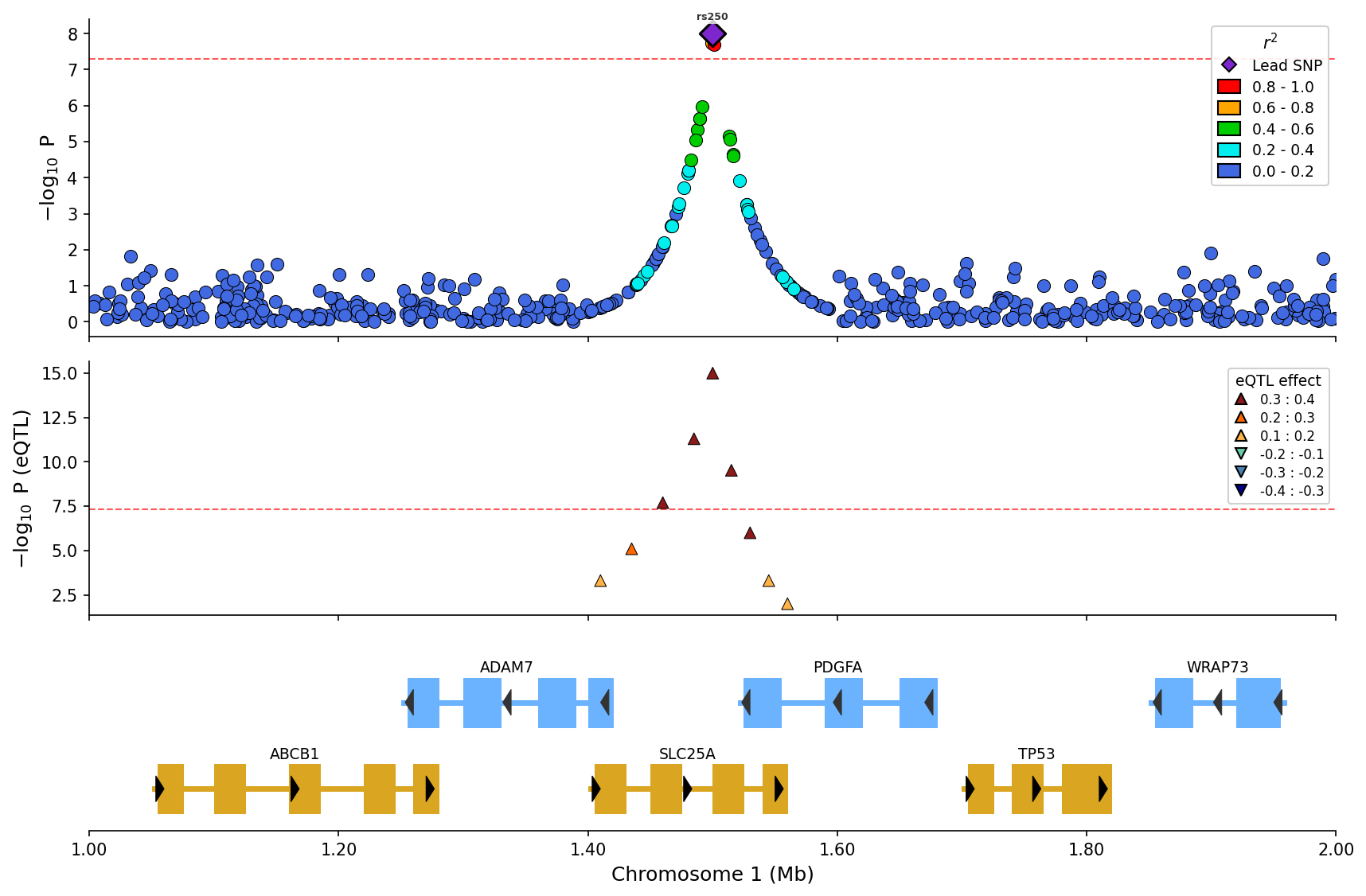
eQTL plot: Expression QTL data aligned with association plots and gene tracks
-
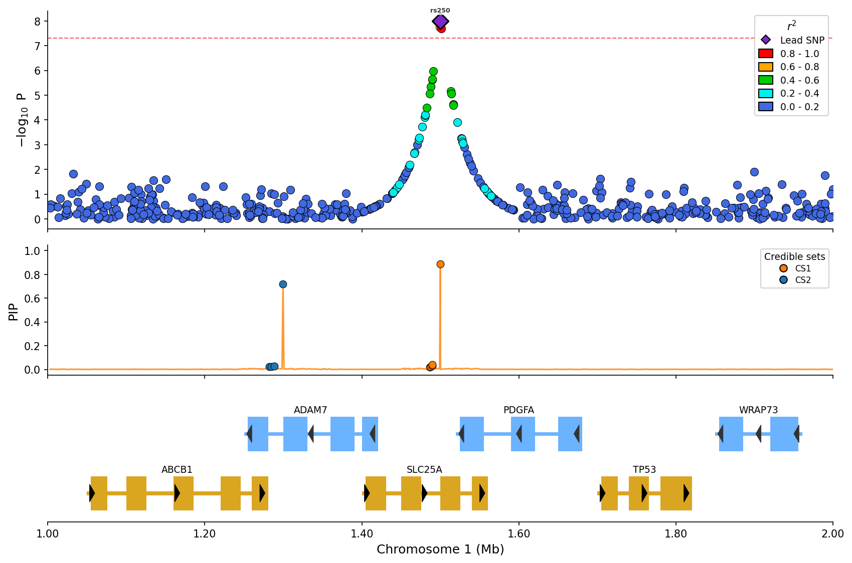
Fine-mapping plots: Visualize SuSiE credible sets with posterior inclusion probabilities
-
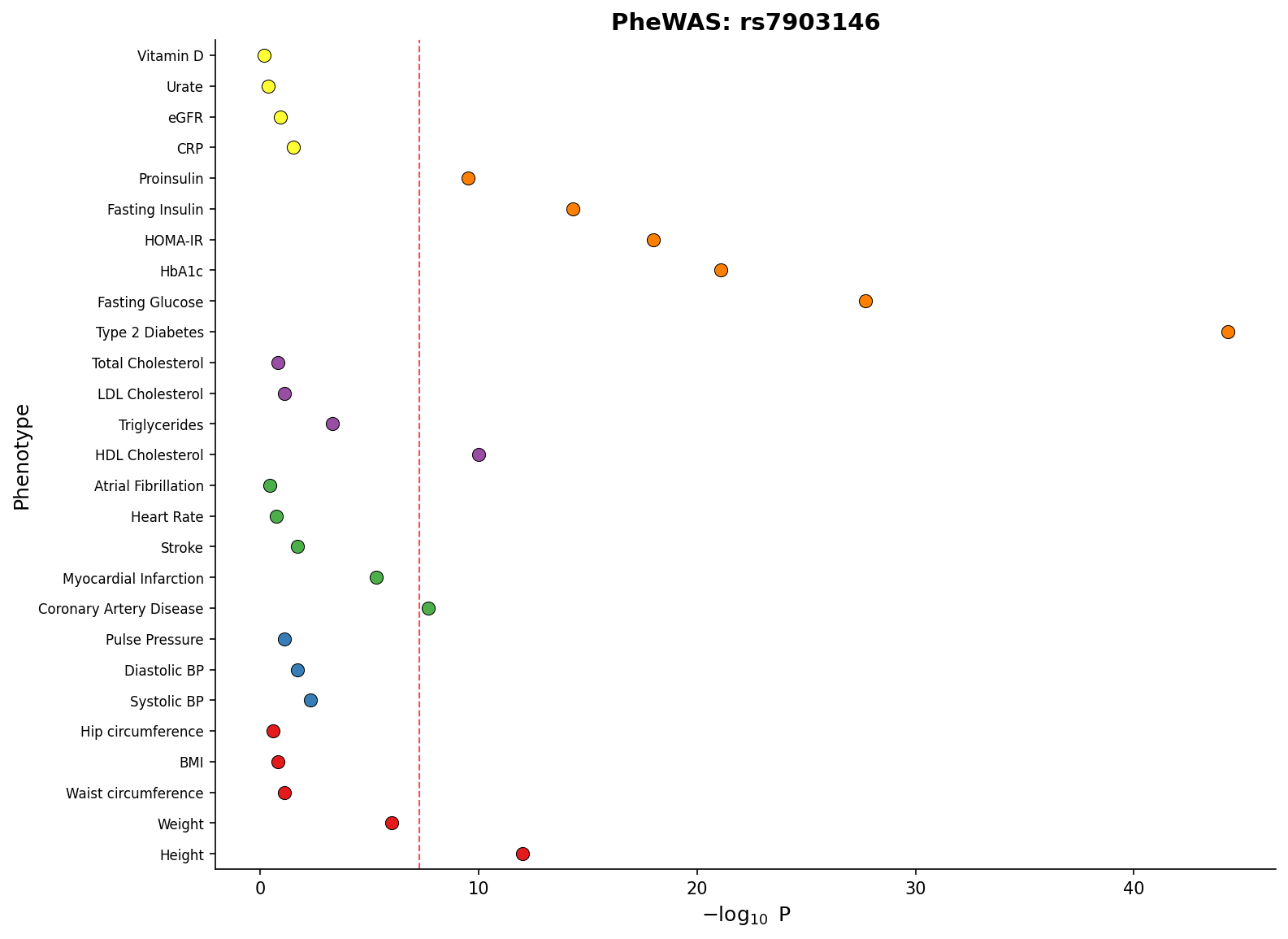
PheWAS plots: Phenome-wide association study visualization across multiple phenotypes
-
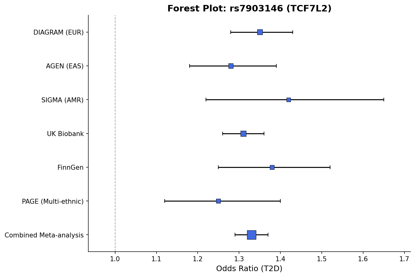
Forest plots: Meta-analysis effect size visualization with confidence intervals
-
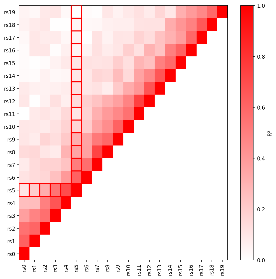
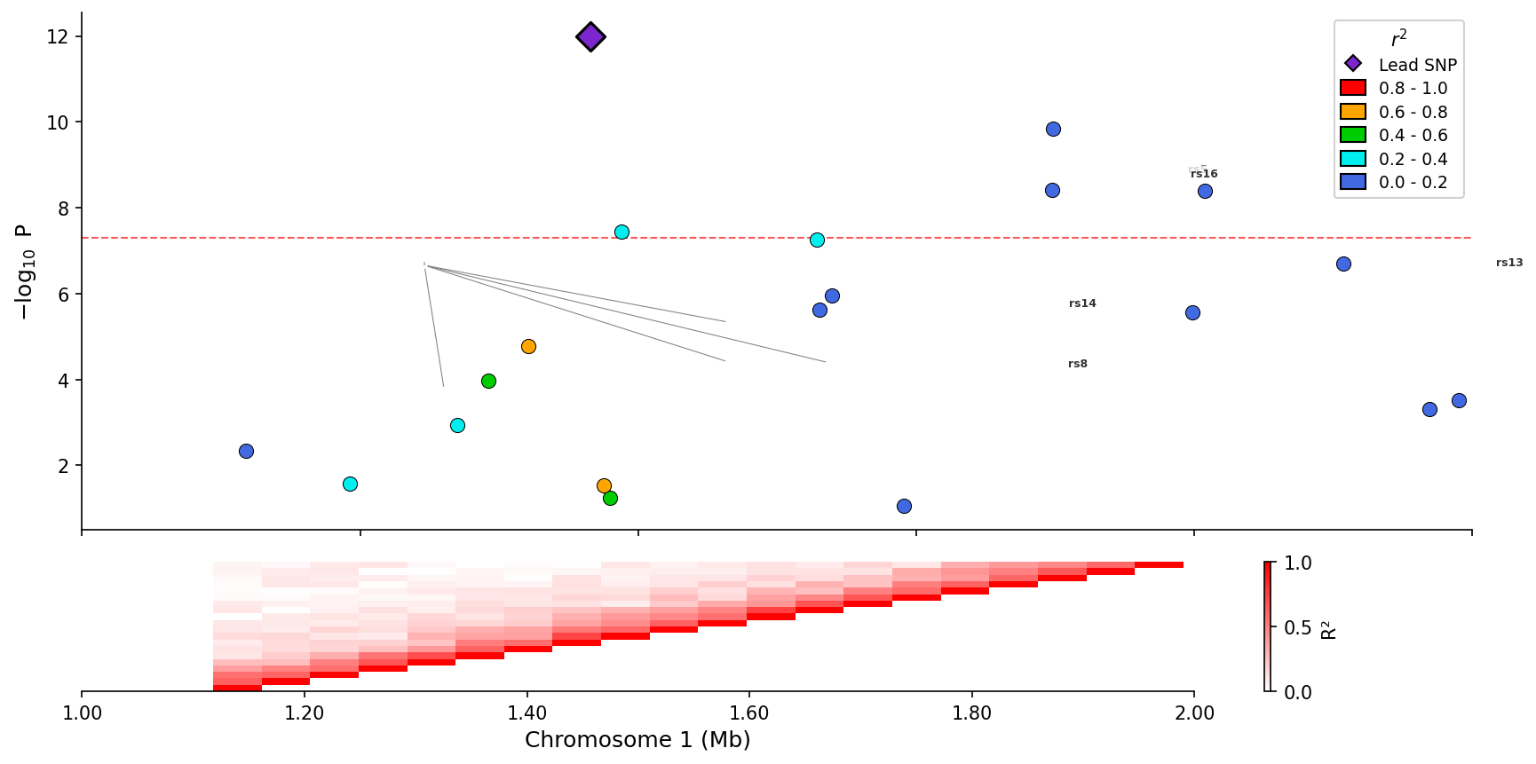
LD heatmaps: Triangular heatmaps showing pairwise LD patterns, standalone or integrated below regional plots
-
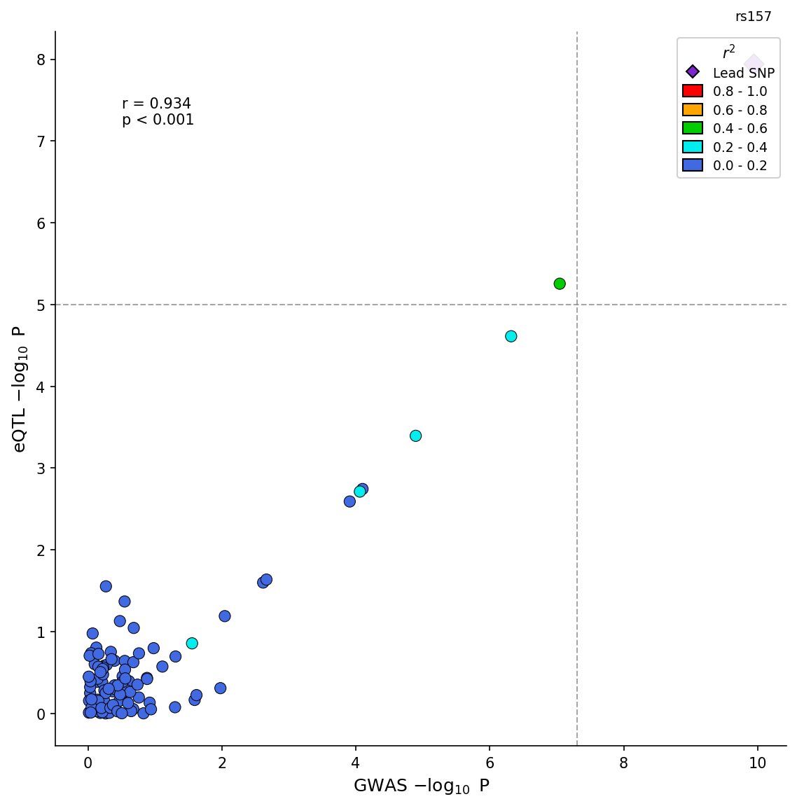
Colocalization plots: GWAS-eQTL scatter plots with LD coloring, correlation statistics, and effect direction visualization
-
Multiple backends: matplotlib (publication-ready), plotly (interactive), bokeh (dashboard integration)
-
Pandas and PySpark support: Works with both Pandas and PySpark DataFrames for large-scale genomics data
-
Convenience data file loaders: Load and validate common GWAS, eQTL and fine-mapping file formats
-
Automatic gene annotations: Fetch gene/exon data from Ensembl REST API with caching (human, mouse, rat, canine, feline, and any Ensembl species)
Installation
pip install pylocuszoom
Or with uv:
uv add pylocuszoom
Or with conda (Bioconda):
conda install -c bioconda pylocuszoom
Quick Start
from pylocuszoom import LDConfig, LocusZoomPlotter

# Initialize plotter (loads reference data for canine)
plotter = LocusZoomPlotter(species="canine", auto_genes=True)

# The region is passed directly; every other option lives on a config model
fig = plotter.plot(
    gwas_df,                        # DataFrame with pos, p_value, rs columns
    chrom=1,
    start=1000000,
    end=2000000,
    ld=LDConfig(lead_pos=1500000),  # Highlight lead SNP
)
fig.savefig("regional_plot.png", dpi=150)
Full Example
from pylocuszoom import (
    ColumnConfig,
    DisplayConfig,
    LDConfig,
    LocusZoomPlotter,
    PanelInputs,
)

plotter = LocusZoomPlotter(
    species="canine",                   # or "feline", or None for custom
    plink_path="/path/to/plink",        # Optional, auto-detects if on PATH
)

fig = plotter.plot(
    gwas_df,
    chrom=1,
    start=1000000,
    end=2000000,
    columns=ColumnConfig(
        chrom_col="chr",                # Column name for chromosome (None: position only)
        pos_col="pos",                  # Column name for position
        p_col="p_value",                # Column name for p-value
        rs_col="rs",                    # Column name for SNP ID
    ),
    display=DisplayConfig(
        show_recombination=True,        # Overlay recombination rate
        snp_labels=True,                # Label top SNPs
        label_top_n=5,                  # How many to label
        figsize=(12, 8),
    ),
    ld=LDConfig(
        lead_pos=1500000,
        ld_reference_file="genotypes",  # PLINK fileset (without extension)
    ),
    panels=PanelInputs(
        genes_df=genes_df,              # Gene annotations
        exons_df=exons_df,              # Exon annotations
    ),
)
The four models are frozen, so a ColumnConfig for your file format or a
PanelInputs holding a gene track can be built once and reused across calls.
Genome Builds
The default genome build for canine is CanFam3.1. For CanFam4 data:
plotter = LocusZoomPlotter(species="canine", genome_build="canfam4")
Recombination maps are automatically lifted over from CanFam3.1 to CanFam4 coordinates using the UCSC liftOver chain file.
Summary statistics on CanFam3.1 can be drawn over CanFam4 genes by passing a chain to plot():
from pylocuszoom import LiftoverConfig

fig = plotter.plot(
    canfam3_gwas_df, chrom=12, start=33_000_000, end=34_000_000,
    liftover=LiftoverConfig(chain_path="canFam3ToCanFam4.over.chain.gz"),
)
See Summary Statistics on Another Build for what is lifted and what is dropped.
Using with Other Species
from pylocuszoom import LocusZoomPlotter

# Feline (LD and gene tracks, user provides recombination data)
plotter = LocusZoomPlotter(species="feline")

# Custom species (provide all reference data)
plotter = LocusZoomPlotter(
    species=None,
    recomb_data_dir="/path/to/recomb_maps/",
)

# Provide data per-plot
fig = plotter.plot(
    gwas_df,
    chrom=1,
    start=1000000,
    end=2000000,
    panels=PanelInputs(recomb_df=my_recomb_dataframe, genes_df=my_genes_df),
)
Automatic Gene Annotations
pyLocusZoom can automatically fetch gene annotations from Ensembl for any species:
from pylocuszoom import LocusZoomPlotter

# Enable automatic gene fetching
plotter = LocusZoomPlotter(species="human", auto_genes=True)

# No need to provide genes_df - fetched automatically
fig = plotter.plot(gwas_df, chrom=13, start=32000000, end=33000000)
Supported species aliases: human, mouse, rat, canine/dog, feline/cat, or any Ensembl species name.
Data is cached locally for fast subsequent plots. Maximum region size is 5Mb (Ensembl API limit).
Genome builds and gene sources
Genes are fetched in the build you set, from whichever source can serve it:
genome_build |
Source | Assembly returned |
|---|---|---|
canfam3.1 (canine default) |
UCSC ncbiRefSeq |
CanFam3.1 |
canfam4, UU_Cfam_GSD_1.0 |
UCSC ncbiRefSeq |
UU_Cfam_GSD_1.0 |
felCat9 (feline default) |
UCSC ncbiRefSeq |
Felis_catus_9.0 |
| anything else | Ensembl REST | Ensembl's current assembly for the species |
Ensembl serves exactly one reference assembly per species and answers a request
naming any other with that same assembly and an HTTP 200, so it cannot supply
CanFam3.1, CanFam4 or FelCat9 and will not say so. Its dog is ROS_Cfam_1.0 and
its cat is F.catus_Fca126_mat1.0. Release 116 was the last on the legacy REST
platform and the archive REST hosts redirect to a help page, so those builds
have no Ensembl source at any URL. UCSC hosts all three, which is where
pyLocusZoom fetches them.
Both sources return the same columns, including an assembly column naming the
assembly each row is in. On the Ensembl path, a genome_build that disagrees
with what Ensembl served warns with a UserWarning naming both.
genome_build also selects the recombination map, where CanFam3.1 and CanFam4
are both supported.
Backends
pyLocusZoom supports multiple rendering backends (set at initialization):
from pylocuszoom import LocusZoomPlotter

# Static publication-quality plot (default)
plotter = LocusZoomPlotter(species="canine", backend="matplotlib")
fig = plotter.plot(gwas_df, chrom=1, start=1000000, end=2000000)
fig.savefig("plot.png", dpi=150)

# Interactive Plotly (hover tooltips, pan/zoom)
plotter = LocusZoomPlotter(species="canine", backend="plotly")
fig = plotter.plot(gwas_df, chrom=1, start=1000000, end=2000000)
fig.write_html("plot.html")

# Interactive Bokeh (dashboard-ready)
plotter = LocusZoomPlotter(species="canine", backend="bokeh")
fig = plotter.plot(gwas_df, chrom=1, start=1000000, end=2000000)
| Backend | Output | Best For | Features |
|---|---|---|---|
matplotlib |
Static PNG/PDF/SVG | Publication-ready figures | Full feature set with SNP labels |
plotly |
Interactive HTML | Web reports, exploration | Hover tooltips, pan/zoom |
bokeh |
Interactive HTML | Dashboard integration | Hover tooltips, pan/zoom |
Note: All backends support scatter plots, gene tracks, recombination overlay, and LD legend. SNP labels (auto-positioned with adjustText) are matplotlib-only; interactive backends use hover tooltips instead.
Plotters prepare data into panel values and put them on one figure plan. Each panel draws itself and one function renders any plan, so panel composition stays consistent while the backend protocol handles drawing primitives.
Breaking in 2.0: custom backends written against 1.x need migration. The
PlotBackendprotocol now carries only drawing primitives; legend and recombination-overlay composition moved above the seam intobackends/composition.py. See docs/ARCHITECTURE.md for the three changes required.
5.0 breaks the protocol again: it drops the members and parameters no caller
used, folds the colour bar into add_heatmap, and hands scatter hover columns
with their roles. docs/MIGRATING-5.0.md
lists each signature change.
SupportsSNPLabels (matplotlib-style repositioned labels) is the one optional
capability, negotiated with a @runtime_checkable protocol: a custom backend
opts in by implementing add_snp_labels and out by omitting it. A backend
without it still renders every regional, Manhattan, Miami, colocalisation, and
PheWAS plot. Heatmaps, error bars, the secondary axis and the region highlight
were optional protocols too until every shipped backend implemented all four;
they are required PlotBackend methods now.
Stacked Plots
Compare multiple GWAS results vertically with shared x-axis:
from pylocuszoom import LocusZoomPlotter, PanelInputs

plotter = LocusZoomPlotter(species="canine")

fig = plotter.plot_stacked(
    [gwas_height, gwas_bmi, gwas_whr],
    chrom=1,
    start=1000000,
    end=2000000,
    panel_labels=["Height", "BMI", "WHR"],
    panels=PanelInputs(genes_df=genes_df),
)
eQTL Overlay
Add expression QTL data as a separate panel. plot() takes the same
PanelInputs for a single GWAS:
from pylocuszoom import EqtlInput, LocusZoomPlotter, PanelInputs

eqtl_df = pd.DataFrame(
    {
        "chr": [1] * 3,
        "pos": [1000500, 1001200, 1002000],
        "p_value": [1e-6, 1e-4, 0.01],
        "gene": ["BRCA1", "BRCA1", "BRCA1"],
    }
)

plotter = LocusZoomPlotter(species="canine")

fig = plotter.plot_stacked(
    [gwas_df],
    chrom=1,
    start=1000000,
    end=2000000,
    panels=PanelInputs(genes_df=genes_df, eqtl=EqtlInput(data=eqtl_df, gene="BRCA1")),
)
Fine-mapping Visualization
Visualize SuSiE or other fine-mapping results with credible set coloring:
from pylocuszoom import FinemappingInput, LocusZoomPlotter, PanelInputs

finemapping_df = pd.DataFrame(
    {
        "chr": [1] * 4,
        "pos": [1000500, 1001200, 1002000, 1003500],
        "pip": [0.85, 0.12, 0.02, 0.45],  # Posterior inclusion probability
        "cs": [1, 1, 0, 2],  # Credible set assignment (0 = not in CS)
    }
)

plotter = LocusZoomPlotter(species="canine")

fig = plotter.plot_stacked(
    [gwas_df],
    chrom=1,
    start=1000000,
    end=2000000,
    panels=PanelInputs(
        genes_df=genes_df,
        finemapping=FinemappingInput(data=finemapping_df, cs_col="cs"),
    ),
)
LD Heatmaps
Create triangular LD heatmaps showing pairwise linkage disequilibrium patterns:
from pylocuszoom import LDHeatmapPlotter

# ld_matrix is a square DataFrame with SNP IDs as index/columns
# snp_ids is a list of SNP IDs in the matrix

ld_plotter = LDHeatmapPlotter()
fig = ld_plotter.plot(
    ld_matrix,
    snp_ids,
    highlight_snp_id="rs12345",  # Highlight lead SNP
    metric="r2",                  # or "dprime"
)
fig.savefig("ld_heatmap.png", dpi=150)
Integrated LD Heatmap with Regional Plot
Add an LD heatmap panel below a regional association plot:
from pylocuszoom import LDConfig, LDHeatmapInput, LocusZoomPlotter, PanelInputs

plotter = LocusZoomPlotter(species="canine")

fig = plotter.plot(
    gwas_df,
    chrom=1,
    start=1000000,
    end=2000000,
    ld=LDConfig(lead_pos=1500000),
    panels=PanelInputs(
        ld_heatmap=LDHeatmapInput(matrix=ld_matrix, snp_ids=snp_ids, height=0.25)
    ),
)
Colocalization Plots
Visualize GWAS-eQTL colocalization by comparing association signals in a scatter plot with LD coloring:
from pylocuszoom import ColocConfig, ColocPlotter

# GWAS and eQTL data with matching positions
gwas_df = pd.DataFrame({
    "pos": positions,
    "p": gwas_pvalues,
    "ld_r2": ld_values,  # Optional: LD with lead SNP
})

eqtl_df = pd.DataFrame({
    "pos": positions,
    "p": eqtl_pvalues,
})

plotter = ColocPlotter()
fig = plotter.plot_coloc(
    gwas_df,
    eqtl_df,
    config=ColocConfig(pos_col="pos", gwas_p_col="p", eqtl_p_col="p", ld_col="ld_r2"),
    gwas_threshold=5e-8,
    eqtl_threshold=1e-5,
)
fig.savefig("colocalization.png", dpi=150)
Advanced options include effect direction coloring and H4 posterior probability display:
fig = plotter.plot_coloc(
    gwas_df,
    eqtl_df,
    config=ColocConfig(
        pos_col="pos",
        gwas_p_col="p",
        eqtl_p_col="p",
        gwas_effect_col="beta",
        eqtl_effect_col="slope",
        color_by_effect=True,  # Green=congruent, Red=incongruent
        h4_posterior=0.85,  # Display coloc H4 probability
    ),
)
PheWAS Plots
Visualize associations of a single variant across multiple phenotypes:
from pylocuszoom import StatsPlotter

phewas_df = pd.DataFrame({
    "phenotype": ["Height", "BMI", "T2D", "CAD", "HDL"],
    "p_value": [1e-15, 0.05, 1e-8, 1e-3, 1e-10],
    "category": ["Anthropometric", "Anthropometric", "Metabolic", "Cardiovascular", "Lipids"],
})

stats_plotter = StatsPlotter()
fig = stats_plotter.plot_phewas(
    phewas_df,
    variant_id="rs12345",
    category_col="category",
)
Forest Plots
Create forest plots for meta-analysis visualization:
from pylocuszoom import StatsPlotter

forest_df = pd.DataFrame({
    "study": ["Study A", "Study B", "Study C", "Meta-analysis"],
    "effect": [0.45, 0.52, 0.38, 0.46],
    "ci_lower": [0.30, 0.35, 0.20, 0.40],
    "ci_upper": [0.60, 0.69, 0.56, 0.52],
    "weight": [25, 35, 20, 100],
})

stats_plotter = StatsPlotter()
fig = stats_plotter.plot_forest(
    forest_df,
    variant_id="rs12345",
    weight_col="weight",
)
Miami Plots
Compare two GWAS datasets with mirrored Manhattan plots (top panel ascending, bottom panel inverted):
from pylocuszoom import MiamiPlotter

plotter = MiamiPlotter(species="human")

fig = plotter.plot_miami(
    discovery_df,
    replication_df,
    top_label="Discovery",
    bottom_label="Replication",
    top_threshold=5e-8,
    bottom_threshold=1e-6,
    highlight_regions=[("6", 30_000_000, 35_000_000)],
)
fig.savefig("miami.png", dpi=150)
Interactive backends (Plotly/Bokeh) provide hover tooltips showing SNP details:
# Plotly - interactive HTML with hover tooltips
plotter = MiamiPlotter(species="human", backend="plotly")
fig = plotter.plot_miami(discovery_df, replication_df, ...)
fig.write_html("miami_interactive.html")

# Bokeh - dashboard-ready interactive plots
from bokeh.io import output_file, save
plotter = MiamiPlotter(species="human", backend="bokeh")
fig = plotter.plot_miami(discovery_df, replication_df, ...)
output_file("miami_bokeh.html")
save(fig)
Manhattan Plots
Create genome-wide Manhattan plots showing associations across all chromosomes:
from pylocuszoom import ManhattanPlotter

plotter = ManhattanPlotter(species="human")

fig = plotter.plot_manhattan(
    gwas_df,
    significance_threshold=5e-8,
    figsize=(12, 5),
)
fig.savefig("manhattan.png", dpi=150)
Categorical Manhattan plots (PheWAS-style) are also supported:
from pylocuszoom import GenomeWideConfig

fig = plotter.plot_manhattan(
    phewas_df,
    category_col="phenotype_category",
    config=GenomeWideConfig(p_col="pvalue"),
)
QQ Plots
Create quantile-quantile plots to assess p-value distribution:
from pylocuszoom import ManhattanPlotter

plotter = ManhattanPlotter()

fig = plotter.plot_qq(
    gwas_df,
    show_confidence_band=True,
    show_lambda=True,
    figsize=(6, 6),
)
fig.savefig("qq_plot.png", dpi=150)
Stacked Manhattan Plots
Compare multiple GWAS results in vertically stacked Manhattan plots:
from pylocuszoom import ManhattanPlotter

plotter = ManhattanPlotter()

fig = plotter.plot_manhattan_stacked(
    [gwas_study1, gwas_study2, gwas_study3],
    panel_labels=["Study 1", "Study 2", "Study 3"],
    significance_threshold=5e-8,
    figsize=(12, 8),
    title="Multi-study GWAS Comparison",
)
fig.savefig("manhattan_stacked.png", dpi=150)
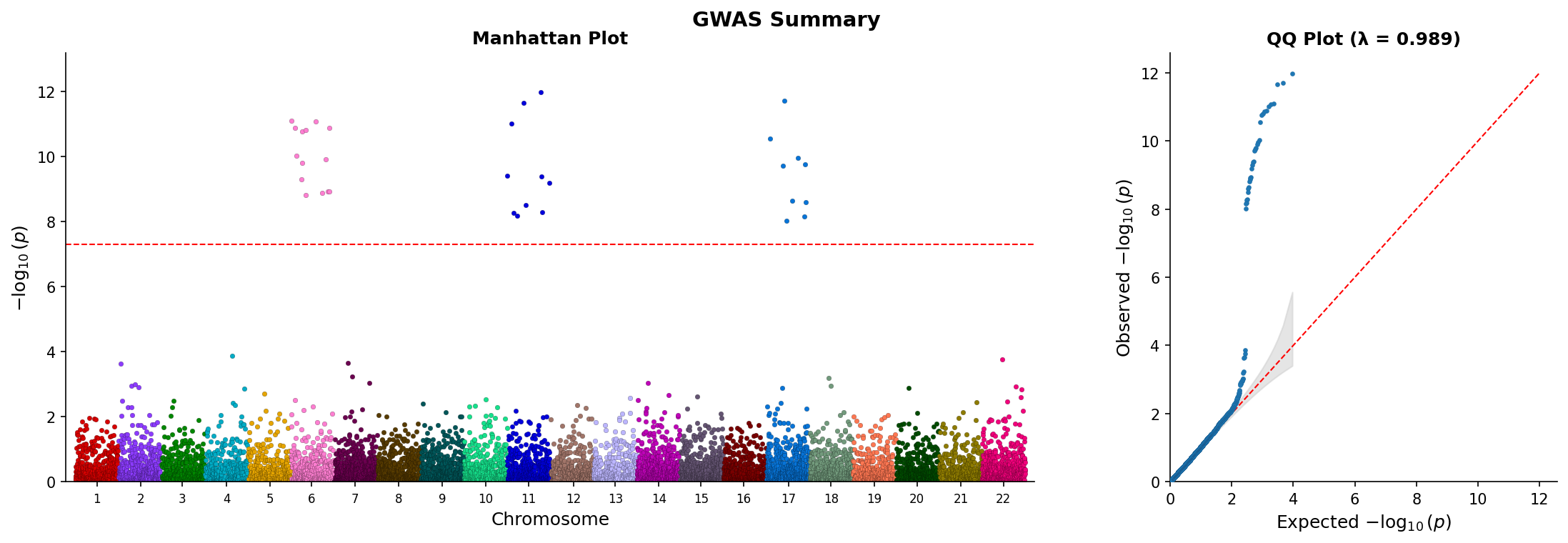
Manhattan and QQ Side-by-Side
Create combined Manhattan and QQ plots in a single figure:
from pylocuszoom import ManhattanPlotter

plotter = ManhattanPlotter()

fig = plotter.plot_manhattan_qq(
    gwas_df,
    significance_threshold=5e-8,
    show_confidence_band=True,
    show_lambda=True,
    figsize=(14, 5),
    title="GWAS Results",
)
fig.savefig("manhattan_qq.png", dpi=150)
suggestive_threshold adds a second line, lambda_gc shows your own inflation factor instead of the computed one, and footer writes a line under both panels.
Every genome-wide method also takes style=GenomeWideStyle(...) for the chromosome palette, point size and alpha, font sizes, chromosome tick step and rotation, and the gap between chromosomes. Unset fields keep the default look. See Styling genome-wide plots.
PySpark Support
Every plot method collects a PySpark DataFrame through to_pandas() before it
reads a single column, so a Spark frame can be passed straight in. Call
to_pandas() yourself when you want to sample a very large frame first:
from pylocuszoom import LocusZoomPlotter, to_pandas

# Passed straight in: the plot method collects it
fig = plotter.plot(spark_gwas_df, chrom=1, start=1000000, end=2000000)

# Sampled first, for a frame too large to collect whole
pandas_df = to_pandas(spark_gwas_df, sample_size=100000)
fig = plotter.plot(pandas_df, chrom=1, start=1000000, end=2000000)
Install PySpark support: uv add pylocuszoom[spark]
Loading Data from Files
pyLocusZoom includes loaders for common GWAS, eQTL, and fine-mapping file formats:
from pylocuszoom import (
    # GWAS loaders
    load_gwas,           # Auto-detect format
    load_plink_assoc,    # PLINK .assoc, .assoc.linear, .qassoc
    load_regenie,        # REGENIE .regenie
    load_bolt_lmm,       # BOLT-LMM .stats
    load_gemma,          # GEMMA .assoc.txt
    load_saige,          # SAIGE output
    # eQTL loaders
    load_gtex_eqtl,      # GTEx significant pairs
    load_eqtl_catalogue, # eQTL Catalogue format
    # Fine-mapping loaders
    load_susie,          # SuSiE output
    load_finemap,        # FINEMAP .snp output
    # Gene annotations
    load_gtf,            # GTF/GFF3 files
    load_bed,            # BED files
)

# Auto-detect GWAS format from filename
gwas_df = load_gwas("results.assoc.linear")

# Or use specific loader
gwas_df = load_regenie("ukb_results.regenie")

# Load gene annotations
genes_df = load_gtf("genes.gtf", feature_type="gene")
exons_df = load_gtf("genes.gtf", feature_type="exon")

# Load eQTL data
eqtl_df = load_gtex_eqtl("GTEx.signif_pairs.txt.gz", gene="BRCA1")

# Load fine-mapping results
fm_df = load_susie("susie_output.tsv")
Data Formats
GWAS Results DataFrame
These are the canonical column names: every load_* function emits them and every
plotter defaults to them, so a loaded frame plots without renaming. Other names,
including the pre-4.0 ps and p_wald, are named through ColumnConfig.
Required columns (names configurable through ColumnConfig):
| Column | Type | Required | Description |
|---|---|---|---|
chr |
str or int | Yes | Chromosome. Selects the plotted region's rows; pass ColumnConfig(chrom_col=None) for a frame already scoped to that chromosome. |
pos |
int | Yes | Genomic position in base pairs (1-based). Must match coordinate system of genes/recombination data. |
p_value |
float | Yes | Association p-value (0 < p ≤ 1). Values are -log10 transformed for plotting. |
rs |
str | No | SNP identifier (e.g., "rs12345" or "chr1:12345"). Used for labeling top SNPs if snp_labels=True. |
Example:
gwas_df = pd.DataFrame({
    "chr": [1, 1, 1],
    "pos": [1000000, 1000500, 1001000],
    "p_value": [1e-8, 1e-6, 0.05],
    "rs": ["rs123", "rs456", "rs789"],
})
Genes DataFrame
| Column | Type | Required | Description |
|---|---|---|---|
chr |
str or int | Yes | Chromosome identifier. Accepts "1", "chr1", or 1. The "chr" prefix is stripped for matching. |
start |
int | Yes | Gene start position (bp, 1-based). Transcript start for strand-aware genes. |
end |
int | Yes | Gene end position (bp, 1-based). Must be >= start. |
gene_name |
str | Yes | Gene symbol displayed in track (e.g., "BRCA1", "TP53"). Keep short for readability. |
Example:
genes_df = pd.DataFrame({
    "chr": ["1", "1", "1"],
    "start": [1000000, 1050000, 1100000],
    "end": [1020000, 1080000, 1150000],
    "gene_name": ["GENE1", "GENE2", "GENE3"],
})
Exons DataFrame (optional)
Provides exon/intron structure. If omitted, genes are drawn as simple rectangles.
| Column | Type | Required | Description |
|---|---|---|---|
chr |
str or int | Yes | Chromosome identifier. |
start |
int | Yes | Exon start position (bp). |
end |
int | Yes | Exon end position (bp). |
gene_name |
str | Yes | Parent gene symbol. Must match gene_name in genes DataFrame. |
Recombination DataFrame
| Column | Type | Required | Description |
|---|---|---|---|
pos |
int | Yes | Genomic position (bp). Should span the plotted region with reasonable density (every ~10kb). |
rate |
float | Yes | Recombination rate in centiMorgans per megabase (cM/Mb). Typical range: 0-50 cM/Mb. |
Example:
recomb_df = pd.DataFrame({
    "pos": [1000000, 1010000, 1020000],
    "rate": [0.5, 2.3, 1.1],
})
Recombination Map Files
When using recomb_data_dir, files must be named chr{N}_recomb.tsv (e.g., chr1_recomb.tsv, chrX_recomb.tsv).
Format: Tab-separated with header row:
| Column | Description |
|---|---|
chr |
Chromosome number (without "chr" prefix) |
pos |
Position in base pairs |
rate |
Recombination rate (cM/Mb) |
cM |
Cumulative genetic distance (optional, not used for plotting) |
chr     pos     rate    cM
1       10000   0.5     0.005
1       20000   1.2     0.017
1       30000   0.8     0.025
Reference Data
Canine recombination maps are downloaded from Campbell et al. 2016 on first use.
To manually download:
from pylocuszoom import download_canine_recombination_maps

download_canine_recombination_maps()
Logging
Logging uses loguru and is off until you turn it on. Importing pyLocusZoom adds and removes no loguru handler, so your application's own logging is untouched. A gene track, recombination overlay or LD colouring the plot has to leave out is a UserWarning, not a log line, so you see it with logging off.
from pylocuszoom import disable_logging, enable_logging

enable_logging()         # INFO and above to stderr
enable_logging("DEBUG")  # for troubleshooting
disable_logging()        # silent again
Requirements
- Python >= 3.10
- matplotlib >= 3.5.0
- pandas >= 1.4.0
- numpy >= 1.21.0
- loguru >= 0.7.0
- plotly >= 5.0.0
- bokeh >= 3.8.2
- kaleido >= 0.2.0 (for plotly static export)
- pyliftover >= 0.4 (for CanFam4 coordinate liftover)
- PLINK 1.9 (for LD calculations) - must be on PATH or specify
plink_path
Optional:
- pyspark >= 3.0.0 (for PySpark DataFrame support) -
uv add pylocuszoom[spark]
Documentation
- Getting Started - Installation and first plot
- User Guide - Comprehensive documentation with API reference
- Configuration - Species flags, recombination caches, LD reference files
- Architecture - Design decisions and component overview
- Code Map - Architecture diagram with source code links
- Development - Dev setup, pre-commit hooks, contributing workflow
- Testing - Running and writing tests
- Example Notebook - Interactive tutorial
- CHANGELOG - Version history
Citation
If you use pyLocusZoom in your research, please cite it. GitHub's "Cite this repository" button reads CITATION.cff, and each GitHub release is archived on Zenodo with its own DOI. The concept DOI 10.5281/zenodo.22665975 always resolves to the latest version.
@software{denyer_pylocuszoom,
  author  = {Denyer, Michael},
  title   = {pyLocusZoom: Python library for multi-species GWAS visualization},
  url     = {https://github.com/michael-denyer/pyLocusZoom},
  doi     = {10.5281/zenodo.22665975},
  license = {GPL-3.0-or-later}
}
License
GPL-3.0-or-later
1 maintainer

Metadata
1 maintainer
Release files for pylocuszoom 5.0.0
For a detailed explanation of source distributions (sdists) and built distributions (wheels), please see the package formats documentation.
Source distribution (sdist)
| File | Size | Uploaded | |
|---|---|---|---|
| pylocuszoom-5.0.0.tar.gz | 26.3 MB | Details |
Built distribution (wheel)
| File | Interpreter | ABI | Platform | Reset |
|---|---|---|---|---|
| pylocuszoom-5.0.0-py3-none-any.whl | Python 3 | none | any | Details |
Total release size: 26.5 MB
Release files / pylocuszoom-5.0.0.tar.gz
| Download URL | pylocuszoom-5.0.0.tar.gz |
|---|---|
| Size | 26.3 MB |
| Tags | Source |
|
SHA-256 checksum How to use checksums |
cc9c83f2e65f7f9c55a0a4853f63d22f2343b598e53c99b25752bcb72d7612e3
|
|
BLAKE2b-256 checksum How to use checksums |
675b47ea44998143902960681780aea08d2728021e474f281c44008a6637cf23
|
| Upload date | |
|
Uploaded using Trusted Publishing? What is trusted publishing? |
Yes |
| Uploaded via |
twine/7.0.0 CPython/3.13.14
|
Provenance
Provenance describes where a file came from. On PyPI, provenance is shared via attestations, which provide a verifiable record of the build or publishing details. View details, limitations and caveats.


PyPI Publish Attestation
PyPI verified that this artifact, at this checksum, originated from the publisher listed below.
Signed by GitHub Actions, verified by PyPI on Sep 23, 2026.
Transparency logRelease files / pylocuszoom-5.0.0-py3-none-any.whl
| Download URL | pylocuszoom-5.0.0-py3-none-any.whl |
|---|---|
| Size | 194.0 kB |
| Tags | Python 3 |
|
SHA-256 checksum How to use checksums |
70d750c3d6606997eeea98207ebaf9b000febb0c335edcf1821f91004c628f02
|
|
BLAKE2b-256 checksum How to use checksums |
7b0083bdb5b01b0a8bd4108e01e74324774b586c4938ce1b850927f8fff67fec
|
| Upload date | |
|
Uploaded using Trusted Publishing? What is trusted publishing? |
Yes |
| Uploaded via |
twine/7.0.0 CPython/3.13.14
|
Provenance
Provenance describes where a file came from. On PyPI, provenance is shared via attestations, which provide a verifiable record of the build or publishing details. View details, limitations and caveats.
PyPI Publish Attestation
PyPI verified that this artifact, at this checksum, originated from the publisher listed below.
Signed by GitHub Actions, verified by PyPI on Sep 23, 2026.
Transparency log













