
pynonthermal




pynonthermal is a Python solver for the Spencer-Fano equation, which describes the energy distribution of non-thermal (fast) electrons slowing down in a plasma. When high-energy leptons — such as the Compton, photoelectric, and pair-production electrons and positrons produced by radioactive decay in supernova ejecta — are injected into a partially ionised gas, they lose energy through three competing channels: Coulomb heating of the free thermal electrons, collisional ionisation, and collisional excitation of bound states.
Given a set of ions (with number densities) and an energy deposition rate, pynonthermal computes:
- the degradation spectrum y(E) of the non-thermal electron population,
- the fraction of deposited energy going to heating, ionisation, and excitation (per channel and per ion),
- non-thermal ionisation rate coefficients for each ion and excitation rate coefficients for individual bound-bound transitions, ready to be used in non-LTE plasma modelling.
These quantities are important, for example, in modelling the late-time spectra and light curves of Type Ia and core-collapse supernovae, where non-thermal ionisation can dominate over photoionisation. The solver follows the method of Kozma & Fransson (1992) (see Method background for details and further references) and ships with the atomic data needed to run out of the box: ionisation cross sections for a wide range of ions, and level/transition data for bound-bound excitation.
Contents
- Installation
- Quick start
- Usage guide
- Complete example: pure-oxygen plasma
- Units and conventions
- Method background
- Cross-section datasets
- Advanced usage: custom excitation cross sections
- Citing pynonthermal
- License
Installation
Released package (recommended for most users):
pip install pynonthermal
Development install with uv:
git clone https://github.com/lukeshingles/pynonthermal.git
cd pynonthermal
uv sync --frozen
source ./.venv/bin/activate
uv pip install --editable .
prek install
Run the test suite with:
uv run -- python3 -m pytest
Quick start
import pynonthermal

sf = pynonthermal.SpencerFanoSolver(emin_ev=1.0, emax_ev=3000.0, npts=4096)

# Add ions that can be non-thermally ionised.
# Here: O II (ion_stage=2, i.e. charge +1) with number density in cm^-3.
sf.add_ionisation(Z=8, ion_stage=2, n_ion=1.0e8)

# Solve for a deposition rate density in eV s^-1 cm^-3.
sf.solve(depositionratedensity_ev=1.0e8)

print("heating fraction:", sf.get_frac_heating())
print("total ionisation fraction:", sf.get_frac_ionisation_tot())
print("total excitation fraction:", sf.get_frac_excitation_tot())
print("sum of fractions:", sf.get_frac_sum())
print("ionisation rate coeff [s^-1]:", sf.get_ionisation_ratecoeff(Z=8, ion_stage=2))
The quickstart notebook contains a fuller worked example, and can be launched on Binder:

Usage guide
All ionisation and excitation channels must be added before calling solve().
1. Create the solver
sf = pynonthermal.SpencerFanoSolver(emin_ev=1.0, emax_ev=3000.0, npts=4096, verbose=False)
emin_ev,emax_ev: bounds of the uniform energy grid in eV. Electrons that degrade belowemin_evare assumed to have thermalised, and their energy is counted as heating.npts: number of energy grid points. More points give better accuracy at the cost of memory and time; checkget_frac_sum()after solving.verbose: print details of the setup, each added channel, and a per-ion, per-shell breakdown during analysis.use_ar1985: use the original Arnaud & Rothenflug (1985) ionisation cross sections (see Cross-section datasets).
The grid is available as sf.engrid (a NumPy array), which is needed if you supply custom excitation cross sections.
2. Add ionisation channels
sf.add_ionisation(Z=8, ion_stage=2, n_ion=1.0e8)
Adds every ionisation shell of the ion to the equation, using the built-in cross-section data. Z is the atomic number, ion_stage is one more than the ion charge (so ion_stage=1 is neutral), and n_ion is the ion number density in cm^-3.
Each ion may be added once; an ion with n_ion=0.0 is silently skipped. If any of the ion's shells has an ionisation potential below emin_ev, a ValueError explains which lower emin_ev to use.
The free electron density is computed automatically from the charges and densities of the added ions (sf.get_n_e()). At least one ionised species (or an explicit override_n_e in solve()) is required.
3. Add excitation channels (optional)
For bound-bound excitation using the built-in atomic database (levels and transitions from the CMFGEN compilation), with LTE level populations at a chosen temperature:
sf.add_ion_ltepopexcitation(Z=8, ion_stage=1, n_ion=1.0e10, temperature=6000)
Optional parameters:
temperature: excitation temperature in K for the LTE Boltzmann level populations (default 3000).maxnlevelslower,maxnlevelsupper: only include transitions from the lowestmaxnlevelslowerlevels up to the lowestmaxnlevelsupperlevels (defaults 5 and 250, matching ARTIS). PassNoneto include all.use_collstrengths: use tabulated collision strengths where available (defaultTrue); otherwise cross sections come from the oscillator strength via the van Regemorter approximation.
Transitions with energies outside the energy grid are dropped. If the internal database has no data for the ion, a ValueError is raised — you can then either supply your own level/transition table via adata_polars or add custom cross sections with add_excitation().
An ion added only for excitation still contributes its charge to the free electron density.
4. Solve
sf.solve(depositionratedensity_ev=1.0e8)
depositionratedensity_ev: the rate of energy deposition per volume in eV s^-1 cm^-3 (must be positive and finite). The energy fractions are independent of this value; the rate coefficients scale linearly with it.override_n_e: optionally override the free electron density (cm^-3) instead of deriving it from the ion populations.
The solution spectrum is stored as sf.yvec over sf.engrid (see Method background for the numerical scheme).
5. Read the results
All getters require solve() to have been called first. Deposition fractions:
sf.get_frac_heating()  # energy fraction to thermal electron heating
sf.get_frac_ionisation_tot()  # energy fraction to ionisation (all ions)
sf.get_frac_excitation_tot()  # energy fraction to excitation (all ions)
sf.get_frac_sum()  # sum of the above; ~1.0 if numerically accurate
sf.get_frac_ionisation_ion(Z, ion_stage)  # one ion's share of the ionisation fraction
Rate coefficients and derived quantities:
sf.get_ionisation_ratecoeff(Z, ion_stage)  # non-thermal ionisation rate coefficient [s^-1]
sf.get_excitation_ratecoeff(Z, ion_stage, transitionkey)  # excitation rate coefficient [s^-1]
sf.get_eff_ionpot(Z, ion_stage)  # effective ionisation potential [eV] (KF92 eq. 12)
sf.get_n_e()  # free (thermal) electron density [cm^-3]
sf.get_n_e_nt()  # non-thermal electron density [cm^-3]
Multiply get_ionisation_ratecoeff() by the ion's number density to get ionisations per second per cm^3, and get_excitation_ratecoeff() by the lower level's population density to get excitations per second per cm^3. For excitations added by add_ion_ltepopexcitation(), the transitionkey is the tuple (lower_level_index, upper_level_index), e.g. (0, 8) for ground level to the eighth excited level.
Call sf.analyse_ntspectrum() (with verbose=True on the solver) to print a detailed per-ion and per-shell breakdown.
6. Plot the solution
sf.plot_yspectrum()  # degradation spectrum y(E)
sf.plot_channels(xscalelog=True)  # energy going to each channel vs electron energy
sf.plot_spec_channels("channels.pdf")  # both panels in one figure, saved to file
Each method shows the figure interactively, or saves it when outputfilename is given; plot_yspectrum() and plot_channels() also accept a Matplotlib axis to draw into an existing figure.
Complete example: pure-oxygen plasma
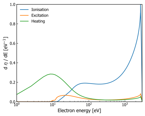
This reproduces Figure 2 of Kozma & Fransson (1992): a pure-oxygen plasma with electron fraction x_e = 0.01, including both ionisation and excitation channels. With verbose=True the solver prints its setup and a per-ion, per-shell breakdown as it runs.
import pynonthermal

n_e = 1e8  # free electron density [cm^-3]
x_e = 1e-2  # ionisation fraction n_OII / (n_OI + n_OII)
n_oxygen = n_e / x_e

ions = [
    # (Z, ion_stage, number_density)
    (8, 1, n_oxygen * (1 - x_e)),  # O I
    (8, 2, n_oxygen * x_e),  # O II
]

sf = pynonthermal.SpencerFanoSolver(emin_ev=1, emax_ev=3000, npts=4096, verbose=True)
for Z, ion_stage, n_ion in ions:
    sf.add_ionisation(Z, ion_stage, n_ion)
    sf.add_ion_ltepopexcitation(Z, ion_stage, n_ion, temperature=6000)

# any positive deposition rate works here: the energy fractions are independent of it
sf.solve(depositionratedensity_ev=2950.49 * n_oxygen)
sf.analyse_ntspectrum()  # print the full breakdown

sf.plot_channels(xscalelog=True)
The resulting plot shows the energy distribution of contributions to ionisation, excitation, and heating; the area under each curve gives the fraction of deposited energy in that channel:
Units and conventions
- Energies are in eV.
- Number densities are in cm^-3.
- Cross sections are in cm^2.
ion_stage = charge + 1(for example, Fe I hasion_stage=1, Fe II hasion_stage=2).depositionratedensity_evinsolve()is in eV s^-1 cm^-3.get_ionisation_ratecoeff()andget_excitation_ratecoeff()both return rates in s^-1.
Method background
The numerical solver is similar to the Spencer-Fano implementation in the ARTIS radiative transfer code (Shingles et al. 2020), itself an independent implementation of Kozma and Fransson (1992, ApJ, 390, 602), based on the electron slowing-down equation of Spencer and Fano (1954, Phys. Rev., 93, 1172). A similar approach is used in CMFGEN.
The integral form of the Kozma and Fransson degradation equation (their equation 7) is discretised on a uniform energy grid as an upper-triangular matrix equation and solved by back-substitution from the highest energy downward. The SpencerFanoSolver class docstring maps each term of the equation to the method that implements it, and the code comments cite the specific Kozma and Fransson equations at each site. The secondary-electron energy distribution follows Opal, Peterson and Beaty (1971) as applied by Kozma and Fransson, and the energy loss rate to thermal electrons uses their Coulomb-logarithm prescription (after Schunk and Hays 1971).
If internal level/transition data are used (for example, via add_ion_ltepopexcitation()), they are imported from the CMFGEN atomic data compilation (see the source data files for references), with excitation cross sections computed from the tabulated collision strengths (Li, Dessart and Hillier 2012, equation 11) or, for permitted transitions without one, from the oscillator strength via the van Regemorter (1962) approximation with the g-bar factor of Mewe (1972), as described in Shingles et al. (2020, section 2.5).
Cross-section datasets
Ionization cross sections from H (Z=1) to Ni (Z=28) use the shell-resolved analytical fits compiled by Arnaud and Rothenflug (1985, A&AS, 60, 425), with updates to Fe from Arnaud and Raymond (1992, ApJ, 398, 394). For heavier elements (Z>28) and any other ions missing from the fit data, the approximation of Axelrod (1980, PhD thesis, Eq. 3.38) is used — the high-energy limit of the Lotz (1967, Z. Phys., 206, 205) formula with relativistic corrections — with subshell binding energies from Lotz (1970, J. Opt. Soc. Am., 60, 206).
Passing use_ar1985=True to the solver selects the original Arnaud and Rothenflug (1985) compilation without the Fe updates, which can be useful for comparison with older published results.
Advanced usage: custom excitation cross sections
You can supply your own excitation cross section table:
sf.add_excitation(Z, ion_stage, levelnumberdensity, xs_vec, epsilon_trans_ev, transitionkey=(lower, upper))
Z: atomic number.ion_stage: one more than ion charge.levelnumberdensity: population density of the lower level (cm^-3), non-negative.xs_vec: NumPy array of cross sections (cm^2), non-negative, defined at every energy insf.engrid(eV).epsilon_trans_ev: transition energy (eV). Must be positive and no greater thanemax_ev, since no electron the solver represents could otherwise drive the transition.transitionkey: any unique key within the ion, used to retrieve the excitation rate coefficient.
Transitions below emin_ev are allowed here, but add_ion_ltepopexcitation() drops them: Kozma and
Fransson (1992) take every electron below emin_ev to have thermalised, so that energy is accounted for
as heating instead.
Retrieve the rate coefficient afterwards with get_excitation_ratecoeff() as in step 5.
Citing pynonthermal
If you use pynonthermal, please cite it via the Zenodo record. Please also consider citing the papers describing the method: Kozma and Fransson (1992) and Shingles et al. (2020).
License
Distributed under the MIT license. See LICENSE for details.
1 maintainer

Download files
Download the file for your platform. If you're not sure which to choose, learn more about installing packages.
Source Distribution
Built Distribution
Filter files by name, interpreter, ABI, and platform.
If you're not sure about the file name format, learn more about wheel file names.
Copy a direct link to the current filters
File details
Details for the file pynonthermal-2026.8.9.tar.gz.
File metadata
- Download URL: pynonthermal-2026.8.9.tar.gz
- Upload date:
- Size: 5.6 MB
- Tags: Source
- Uploaded using Trusted Publishing? Yes
- Uploaded via:
twine/7.0.0 CPython/3.13.14
File hashes
| Algorithm | Hash digest | |
|---|---|---|
| SHA256 |
00d8feea4c3ee201c3233725b20e66b478e31d4709baa8d39013fa0fc42e518b
|
|
| MD5 |
e3bd24fd09195d3b6f7fe1f85e7f46ad
|
|
| BLAKE2b-256 |
ee36cf701efaa92836afcc5cde1f2318ba37be2702290a84bb5484d05535f782
|
Provenance
The following attestation bundles were made for pynonthermal-2026.8.9.tar.gz:
Publisher:
deploypypi.yml on lukeshingles/pynonthermal
-
Statement:
-
Statement type:
https://in-toto.io/Statement/v1 -
Predicate type:
https://docs.pypi.org/attestations/publish/v1 -
Subject name:
pynonthermal-2026.8.9.tar.gz -
Subject digest:
00d8feea4c3ee201c3233725b20e66b478e31d4709baa8d39013fa0fc42e518b - Sigstore transparency entry: 2399701877
- Sigstore integration time:
-
Permalink:
lukeshingles/pynonthermal@aaab13c2e90ed14e4465001dc064112dc86d821a -
Branch / Tag:
refs/tags/v2026.8.9 - Owner: https://github.com/lukeshingles
-
Access:
public
-
Token Issuer:
https://token.actions.githubusercontent.com -
Runner Environment:
github-hosted -
Publication workflow:
deploypypi.yml@aaab13c2e90ed14e4465001dc064112dc86d821a -
Trigger Event:
release
-
Statement type:
File details
Details for the file pynonthermal-2026.8.9-py3-none-any.whl.
File metadata
- Download URL: pynonthermal-2026.8.9-py3-none-any.whl
- Upload date:
- Size: 5.5 MB
- Tags: Python 3
- Uploaded using Trusted Publishing? Yes
- Uploaded via:
twine/7.0.0 CPython/3.13.14
File hashes
| Algorithm | Hash digest | |
|---|---|---|
| SHA256 |
350da28e33027f10c43a623e13656018ba5fa980f745ce2d0060c8e44c89649f
|
|
| MD5 |
bdee58b817ec966220f09a4f86099717
|
|
| BLAKE2b-256 |
9d2e7c76e127ab2a42c7d5de7e946f5c683bdf96fc0d3f88b1a63ed3d4b4dc44
|
Provenance
The following attestation bundles were made for pynonthermal-2026.8.9-py3-none-any.whl:
Publisher:
deploypypi.yml on lukeshingles/pynonthermal
-
Statement:
-
Statement type:
https://in-toto.io/Statement/v1 -
Predicate type:
https://docs.pypi.org/attestations/publish/v1 -
Subject name:
pynonthermal-2026.8.9-py3-none-any.whl -
Subject digest:
350da28e33027f10c43a623e13656018ba5fa980f745ce2d0060c8e44c89649f - Sigstore transparency entry: 2399702099
- Sigstore integration time:
-
Permalink:
lukeshingles/pynonthermal@aaab13c2e90ed14e4465001dc064112dc86d821a -
Branch / Tag:
refs/tags/v2026.8.9 - Owner: https://github.com/lukeshingles
-
Access:
public
-
Token Issuer:
https://token.actions.githubusercontent.com -
Runner Environment:
github-hosted -
Publication workflow:
deploypypi.yml@aaab13c2e90ed14e4465001dc064112dc86d821a -
Trigger Event:
release
-
Statement type:







