Information-theoretic reconstruction of quantum wavefunctions from discrete bitstrings

Project description
QBitwave
Python class to model quantum-like dynamics as the deterministic evolution of compressibility in finite bitstrings.
Install
pip install qbitwave
https://pypi.org/project/qbitwave/
Description
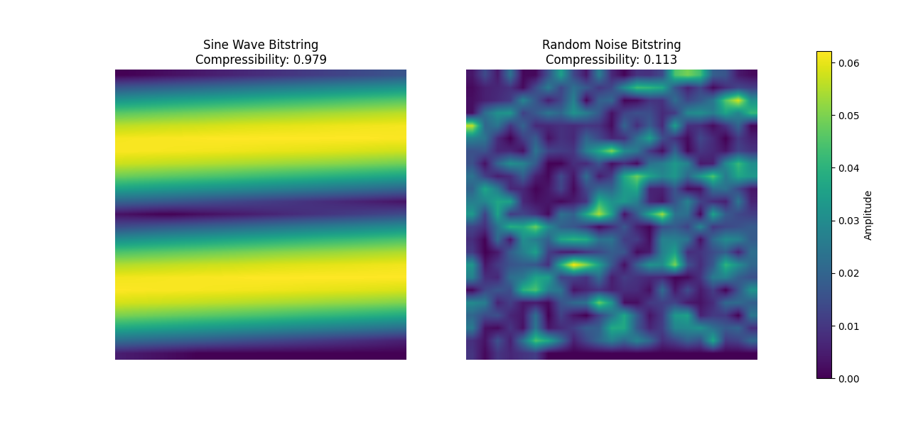
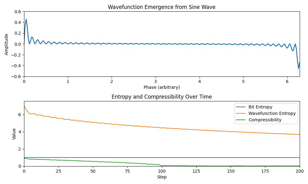
The wavefunction ψ is interpreted not as a physical field but as the minimal compression algorithm that reproduces a given informational state. Existence corresponds to compressibility — the most compressible configurations dominate.
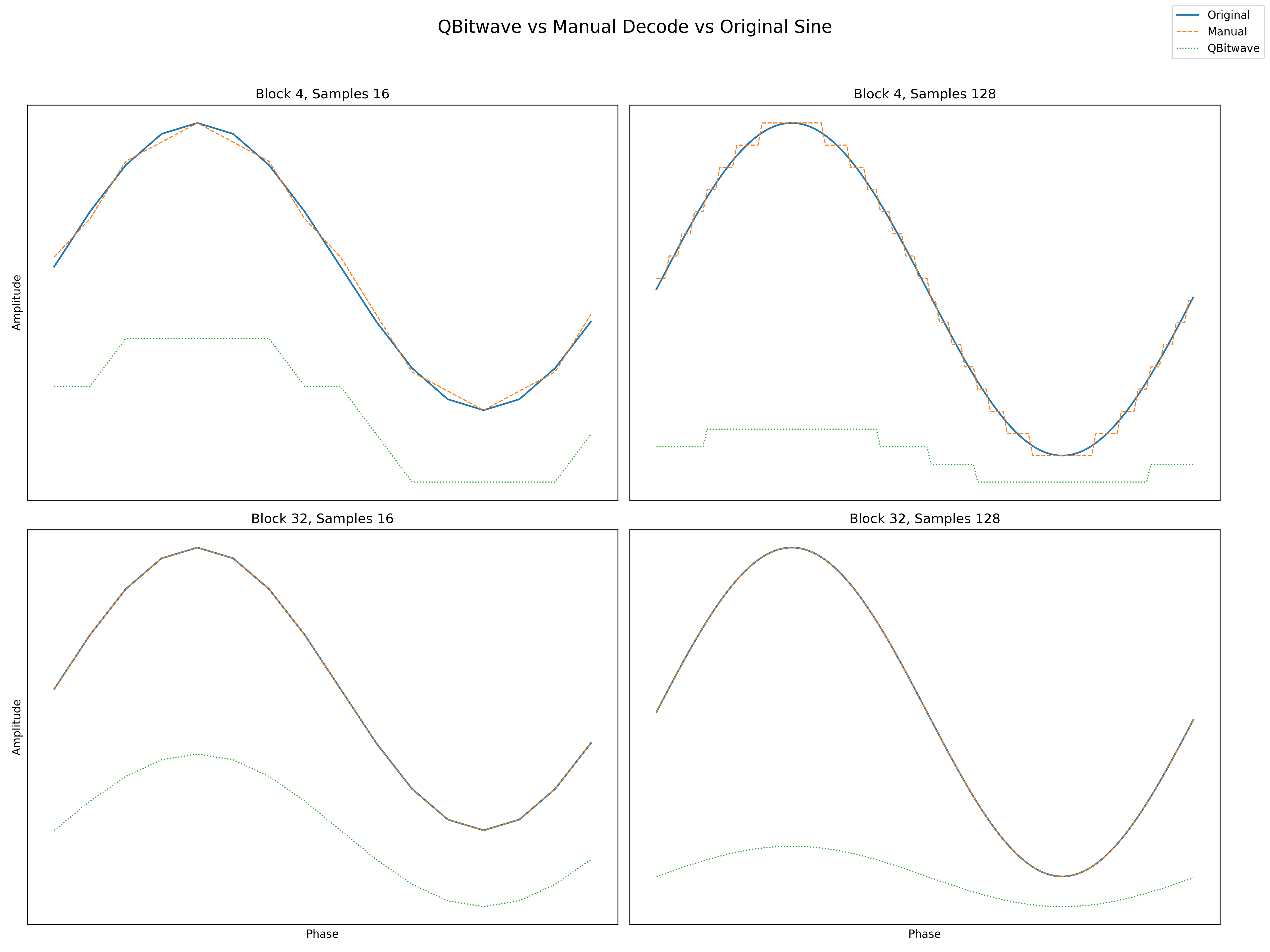
A finite bitstring encodes a discretized wavefunction, which can be reconstructed as normalized complex amplitudes. Conceptually, the bitstring is like a “measurement” of the wavefunction: many wavefunctions may correspond to the same bitstring, but each wavefunction carries richer structure in amplitude and phase.
Through Fourier-domain transformations and entropy measures, QBitwave unifies bitstrings, complex amplitudes, and probabilistic behavior into a single information-centric framework.
Fundamental Principles
- Compression → quantum probability amplitude → predictability (smooth, emergent laws of physics)
- Smooth, regular data compresses well → high amplitude in few Fourier components (low entropy)
- Random/noisy data is incompressible → low amplitude concentration
- Wavefunction = minimal spectral description reproducing the bitstring
- Phase structure contributes to wavefunction complexity; rapid phase variation increases informational cost
Features
- Forward mapping: wavefunction → bitstring
- Reverse mapping: bitstring → minimal complex wavefunction
- Phase-aware spectral complexity measure (
wave_complexity()) - Block-size selection via entropy maximization
- Shannon entropy computation
- Fourier-based compressibility measure reflecting structure
- Deterministic evolution driven by minimal spectral complexity
QBitwaveMDL
This is new rewritten version of QBitwave, with refined spectral complexity measure and old experimental and legacy code stripped.
QBitSpinor
QBitSpinor extends the spectral informational framework to two-component spinor fields, enabling representation of internal degrees of freedom (analogous to spin-½ systems) within the same MDL-based formalism.
While QBitwaveMDL models a scalar complex field ψ(x), QBitSpinor models a vector-valued wavefunction:
ψ(x) = (ψₐ(x), ψᵦ(x))
Each component is encoded spectrally, and structural complexity is computed over the combined power of both components.
| Conceptual Relation |
|---|
QBitwaveMDL → Scalar informational field |
QBitSpinor → Internal structure (spinor / identity encoding) |
Interpretation
- A spinor is not treated as a physical object, but as a more expressive compression scheme
- Two components allow encoding of relational or identity-preserving structure
- The additional degrees of freedom enable:
- Representation of distinguishability under compression
- Emergence of exclusion-like behavior (via structural constraints)
- Mapping to Bloch sphere representation
In this framework:
- Scalar fields compress geometry
- Spinors compress identity
Structural Complexity
The spectral complexity generalizes to:
C_Q = Σ k_eff² (|Aₐ(k)|² + |Aᵦ(k)|²)
This reflects the total informational cost of encoding both components.
Bloch Representation
The internal structure can be mapped to a Bloch vector:
- Ex = 2 Re(ψₐ* ψᵦ)
- Ey = 2 Im(ψₐ* ψᵦ)
- Ez = |ψₐ|² − |ψᵦ|²
This provides a geometric interpretation of the internal state.
Features
- Two-component spectral encoding (α, β)
- FFT-based mode extraction
- Joint spectral complexity measure
- Wavefunction reconstruction ψ(x) ∈ ℂ²
- Bloch vector computation
- MDL-based description length estimation
- Typicality weighting via exp(-λ C_Q)
Example Usage
import numpy as np
from qbitwave.qbitspinor import QBitSpinor

N = 32
spinor = QBitSpinor(N)

# Define spinor components
alpha = np.exp(1j * np.linspace(0, 2*np.pi, N))
beta  = np.exp(-1j * np.linspace(0, 2*np.pi, N))

# Encode into spectral modes
spinor.encode(alpha, beta)

# Evaluate wavefunction
psi = spinor.evaluate()  # shape (N, 2)

# Compute Bloch vectors
bloch = spinor.get_bloch_vectors()

# Complexity and typicality
C = spinor.spectral_complexity()
w = spinor.typicality_weight()


### QBitwaveND

Experimental. `QBitwaveND` generalizes `QBitwave` to **N-dimensional continuous fields** and allows **dynamical evolution in time**.


| Conceptual Relation |
|--------------------|
| `QBitwave` → Emergence: bitstring → ψ(x) |
| `QBitwaveND` → Evolution: ψ(x) → ψ(x, t) |

`QBitwaveND` applies unitary, physically motivated evolution consistent with the **Schrödinger free-particle dispersion relation**, but framed entirely **informationally**:

1. Take N-dimensional complex amplitude array ψ(x₁, x₂, …, xₙ)
2. Compute Fourier transform:
   ψ̃(k) = FFT[ψ(x)] / ∏ shape
3. Apply time evolution in frequency space:
   ψ̃(k, t) = ψ̃(k) · exp(-i·ω(k)·t), where ω(k) = (ħ |k|²) / 2m
4. Inverse transform to get ψ(x, t)

**Interpretation:**

- Time is an informational parameter — the **phase evolution of encoded structure**
- Provides **unitary time evolution over emergent informational geometry**, extending static ψ(x) of `QBitwave` to ψ(x, t)

**Attributes:**

- `amplitudes` : N-dimensional complex array ψ(x) at t=0
- `shape` : spatial dimensions of the array
- `ndim` : number of spatial dimensions
- `fft_coeffs` : normalized Fourier coefficients ψ̃(k)
- `freqs` : per-axis frequency arrays
- `mass` : effective mass parameter (ħk² / 2m)
- `c` : speed of light (for optional relativistic corrections)
- `hbar` : reduced Planck constant

**Key Methods:**

- `from_array(data_array)` : construct from existing N-D array
- `from_qbitwave(qb: QBitwave)` : create N-D field from a 1D informational wavefunction
- `time_evolve_coeffs(t)` : return Fourier coefficients after time evolution
- `evaluate(*coords, t=0.0)` : compute ψ(x, t) at arbitrary coordinates
- `probability(*coords, t=0.0)` : return |ψ(x, t)|² (Born-rule analog)


## Example Usage

```python
from qbitwave import QBitwave, QBitwaveND

# Create a 1D informational wavefunction
qb = QBitwave("010110110001")

# Lift it to N-dimensional dynamic field
qn = QBitwaveND.from_qbitwave(qb)

# Evaluate amplitude at x=0.2, t=0.5
psi_t = qn.evaluate(0.2, t=0.5)

# Compute probability (Born rule analog)
P = qn.probability(0.2, t=0.5)
Images
Release history Release notifications | RSS feed


Download files
Download the file for your platform. If you're not sure which to choose, learn more about installing packages.
Source Distribution
Built Distribution
Filter files by name, interpreter, ABI, and platform.
If you're not sure about the file name format, learn more about wheel file names.
Copy a direct link to the current filters
File details
Details for the file qbitwave-0.3.5.tar.gz.
File metadata
- Download URL: qbitwave-0.3.5.tar.gz
- Upload date:
- Size: 24.5 kB
- Tags: Source
- Uploaded using Trusted Publishing? No
- Uploaded via: twine/6.1.0 CPython/3.12.3
File hashes
| Algorithm | Hash digest | |
|---|---|---|
| SHA256 |
57e25634d6e06caaa109706697e12020ef80603a52348e3859558cb604d82581
|
|
| MD5 |
a636ab9f2673899403d0002e71f5ae44
|
|
| BLAKE2b-256 |
15ae85ae4c97bcbb2bdf4415ebfdf34fa9ad543c989ce496dc31825032a27508
|
File details
Details for the file qbitwave-0.3.5-py3-none-any.whl.
File metadata
- Download URL: qbitwave-0.3.5-py3-none-any.whl
- Upload date:
- Size: 20.7 kB
- Tags: Python 3
- Uploaded using Trusted Publishing? No
- Uploaded via: twine/6.1.0 CPython/3.12.3
File hashes
| Algorithm | Hash digest | |
|---|---|---|
| SHA256 |
4ee5c53452b5c005bdbf0e881352626a52a5eeb916bb64170ec9533efef0ce43
|
|
| MD5 |
1d2e9c37e87a0075ec80e195def2f699
|
|
| BLAKE2b-256 |
9aabe0ba497473f33a277e4c3cd212feec34eb4d4bf6ecb64e0e199f55640828
|


