
qthermo
Thermodynamic bookkeeping for open quantum systems — heat, work, entropy production, currents and their fluctuations — with the modelling traps checked for you.
You write down a Hamiltonian and the baths. qthermo gives you per-bath heat
currents, entropy production, efficiencies against their Carnot bounds,
site-resolved energy flows, exact current fluctuations and uncertainty-relation
ratios, for stroke machines and continuous machines, from one qubit to a few
hundred levels. It also tells you when the model you wrote down cannot mean
what you think it means.
pip install "qthermo[plot]"        # numpy, scipy, matplotlib
python -m qthermo.benchmarks      # 44 checks against published results, ~40 s
For the latest version, pip install "qthermo[plot] @ git+https://github.com/VivekKhanna0/Qthermo".
To run the examples and tests, git clone the repository and
pip install -e ".[dev]".
Highlights, each reproduced by the package and checked in CI:
- Local master equations can make heat flow from cold to hot.
qthermodetects it and runs the same machine under global baths in one call. - The three-qubit absorption fridge hits COP = ω_c/ω_h to 1e-15, and its target qubit transiently cools below its steady state.
- The coherently driven maser beats the classical thermodynamic uncertainty relation (exact current noise, no sampling).
- Optimal finite-time protocols for any drive: simulations land on the predicted minimum L²/τ to 0.2%.
- A quantum Szilard engine attains the Sagawa–Ueda bound exactly, and a zz-coupled transistor amplifies heat currents 4.8×.
- Which master equation is right? For coupled oscillators, where the exact answer is known, the global equation is off by 25× at weak coupling and the local one by 10% when detuned. The Redfield bath matches exact to 0.1% in both regimes.
- Agrees with QuTiP to 1e-16 (steady states) and 1e-10 (dynamics).
New here? examples/tutorial.ipynb takes one
research question (a two-qubit thermal diode) from a Hamiltonian to publishable
numbers, including the checks a referee would ask about. It renders on GitHub
with all outputs.
Docs: physics definitions · API reference · figure gallery · examples · changelog
Reproduce a paper in 10 lines
A question papers in this field argue about: the local and global master equations give different heat currents, so which one is right? For two coupled oscillators the exact answer is known, so each can be graded:
import qthermo as qt

r = qt.papers.local_vs_global(detuning=0.1)   # Hofer et al., NJP 19, 123037 (2017)
print(r.report())
r.plot()
     local: worst error   10.3%
    global: worst error    4.0%
  redfield: worst error    0.0%
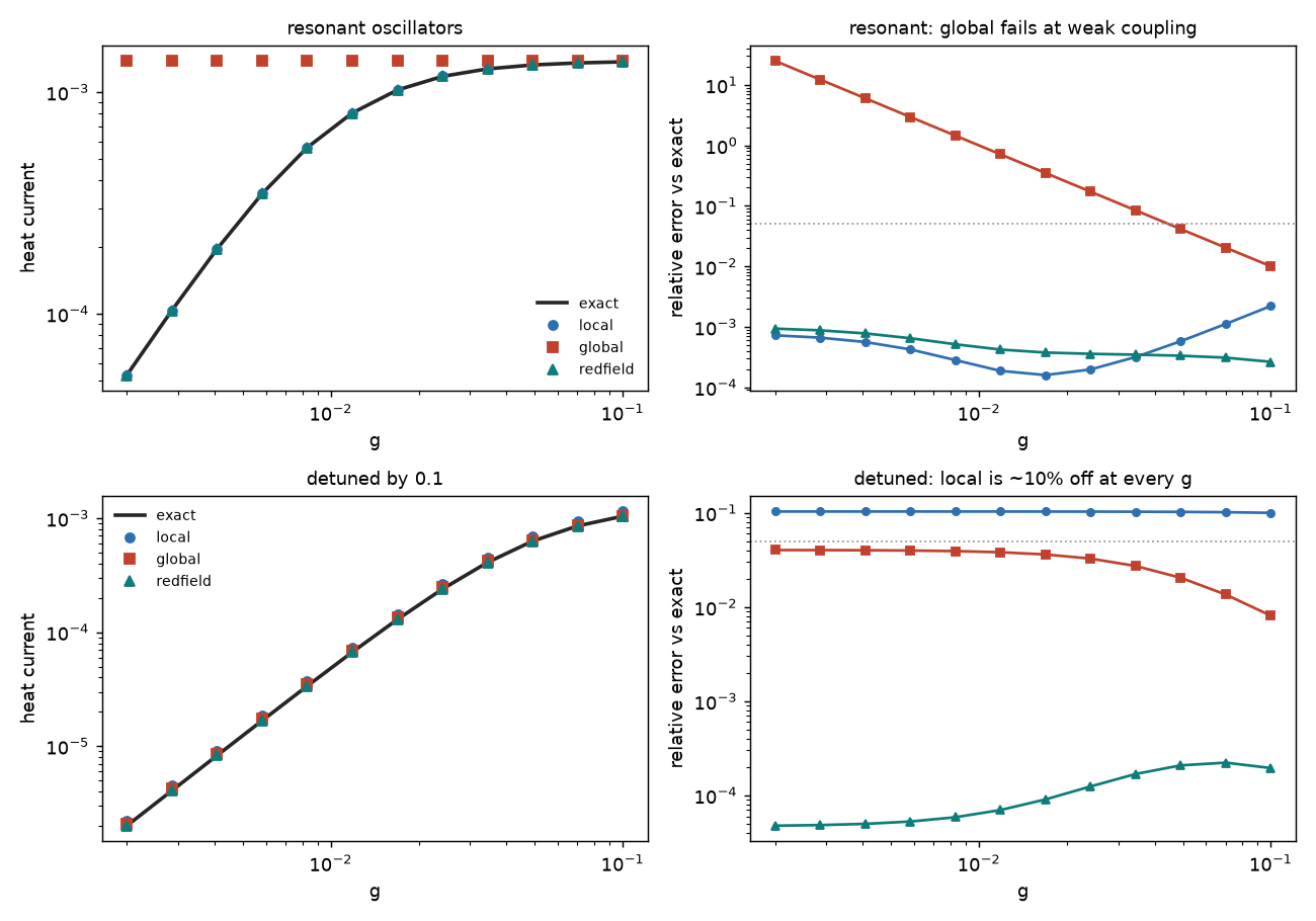
Each standard approximation fails somewhere (top: global, for resonant
oscillators at weak coupling; bottom: local, for detuned ones). The Redfield
bath (qt.redfield_bath) is right in both cases. The same three baths work on
any Hamiltonian you write down, so you can run this check on your own model:
see Your own model. The script that draws this figure is
examples/reproduce_local_vs_global.py.
Thirty seconds
import qthermo as qt

fridge = qt.models.absorption_refrigerator(T_c=1.0, T_h=6.0, T_r=1.5)
steady = fridge.analyze()
print(steady.report())
bath                  T   J (into system)          -J/T
-------------------------------------------------------
cold                  1      6.963227e-04   -6.9632e-04
hot                   6      2.088968e-03   -3.4816e-04
room                1.5     -2.785291e-03    1.8569e-03
-------------------------------------------------------
sum                             1.301e-18    8.1238e-04
entropy production rate: 8.1238e-04
note: local baths -- valid only for inter-site coupling << bath rates; compare with global baths
steady.cop("cold", "hot")                                  # 0.3333 = w_c / w_h exactly
steady.absorption_carnot_cop("cold", "hot", "room")        # 1.5
print(fridge.compare().report())       # would "you used a local master equation" change anything?
bath                 J local      J global   rel. diff
------------------------------------------------------
cold             6.96323e-04   7.53796e-04       7.62%
hot              2.08897e-03   2.27304e-03       8.10%
room            -2.78529e-03  -3.02684e-03       7.98%
------------------------------------------------------
entropy production rate: local 8.1238e-04, global 8.8526e-04
steady-state trace distance: 1.040e-02
qt.plot_machine(steady) # the figure below

Baths (squares) and qubits (circles) share one temperature colour scale; each qubit is coloured by its virtual temperature. The cold qubit is colder than every bath, which nothing passive can do. Arrow widths are heat currents, and the internal balances close to ~1e-17.
Your own model
Nothing above is special-cased. Describe the sites, the couplings and which bath touches which site:
machine = qt.build_model(
    local_H=[qt.qubit_hamiltonian(1.0), qt.qubit_hamiltonian(0.6)],
    interactions={(0, 1): (0.3 * qt.sigma_x, qt.sigma_x)},          # 0.3 sx (x) sx
    baths=[dict(name="hot", site=0, coupling=qt.sigma_x, T=2.0, gamma=0.1),
           dict(name="cold", site=1, coupling=qt.sigma_x, T=1.0, gamma=0.1)],
    master_equation="global")

steady = machine.analyze()                          # exact steady state, per-bath currents
print(qt.audit(machine))                            # every consistency check
machine.compare()                                   # the same machine under local baths
qt.current_statistics(machine, "hot")               # exact noise, TUR / KUR ratios
qt.plot_machine(steady)                             # heat-flow network, virtual temperatures
qt.report(machine, "machine.html")                  # all of it in one shareable page
Sites can have any dimension, and interactions can be given as full matrices.
For full control, build the baths yourself:
qt.davies_bath(H, coupling, T) gives the global (secular,
detailed-balance) bath for any Hamiltonian, coupled, degenerate or many-body,
and qt.local_bath gives the local one. qt.analyze(H, baths) takes any list
of them. QuTiP Qobjs are accepted anywhere an array is.
I want to...
| ...do this | call |
|---|---|
| get currents, entropy production, COP/efficiency of a continuous machine | qt.analyze(H, baths) or model.analyze() |
| check my model for known modelling mistakes | qt.audit(model) or qt.audit(H, baths) |
| describe my own machine once and get every tool | qt.build_model(local_H, interactions, baths) |
| check which master equation is right for my model | model.rebuild("redfield").analyze() against model.compare(); see qt.papers.local_vs_global() |
| build baths for a coupled / many-body system | qt.davies_bath (global), qt.local_bath (local) |
| know whether local vs global master equations matter | model.compare() |
| see where heat flows inside a multi-qubit machine | qt.heat_flow_map(steady), qt.plot_machine(steady) |
| follow each qubit (energy, T*, entanglement) through a cycle | qt.site_dynamics(result, dims, local_H), qt.plot_site_dynamics |
| get the noise of a current and the TUR/KUR ratios | qt.current_statistics(model, "bath") |
| simulate a stroke cycle and its limit cycle | qt.Cycle([qt.Stroke(...), ...]).limit_cycle(rho0) |
| know the quasi-static limit of an interacting Otto engine | qt.ideal_otto(H_c, H_h, T_c, T_h) |
| get the exact heat distribution of one cycle | qt.cycle_counting(cycle, {"stroke": "quanta"}) |
| map engine / fridge / heater / accelerator regions | qt.mode_map(build, xs, ys), qt.plot_mode_map |
| scan any machine over parameters | qt.sweep, qt.scan_2d, qt.pareto_front |
| go beyond weak coupling | qt.reaction_coordinate_model, qt.rc_convergence |
| cost of erasure and the optimal protocol | qt.landauer_erasure, qt.geodesic_schedule |
| work from information (measurement + feedback) | qt.szilard_engine(T, error=..., tau=...) |
| the least-dissipative schedule for my drive | qt.optimal_schedule(H_of, baths_of, T, path) |
| a machine powered by a periodic drive | qt.floquet_analyze(H_of_t, period, [qt.DrivenBath(...)]) |
| what happens after switching a machine on | qt.transient(model, rho0, duration) |
| conductance matrix, Onsager check, transistor gain | qt.response(build, {bath: T}) |
| analyse a quantum battery | qt.batteries.ergotropy_split, locked_ergotropy, dicke_battery |
| use lab numbers (GHz, mK, µs, W) | lab = qt.LabUnits(5.0); lab.temperature(20), lab.rate(1/T1), lab.to_watts(J) |
| save results with provenance | qt.save(result, "file.json") |
| send a colleague the result and the checks | qt.report(model, "machine.html"), a single self-contained page |
| an interactive page with a parameter slider | qt.explorer(build, values, path="x.html") |
| confirm the package is right | python -m qthermo.benchmarks |
What it catches
Most of the value is here. Each of these is a mistake that produces a plausible
number with no error message, and each is detected and explained. qt.audit
runs every check in one call:
print(qt.audit(qt.models.two_qubit_heat_valve(master_equation="local")))
[ERROR] local vs global: the two master equations disagree on the direction of heat flow for hot, cold
          Inter-site coupling is too strong for the local approximation. Use the
          global model.
[info]  relaxation time: 2.72 (populations)
[ok]    steady state: unique
[ok]    second law: entropy production rate 1.937e-02 >= 0
[ok]    internal currents: site energy balances close to 3.5e-17
[ok]    uncertainty relation: 'hot': TUR ratio 9.626 >= 2
[ok]    uncertainty relation: 'cold': TUR ratio 5.117 >= 2
------------------------------------------------------------
1 error(s), 0 warning(s), 6 other checks
| Trap | What happens | What qthermo does |
|---|---|---|
| Local master equation on coupled sites | Heat can flow cold → hot; σ < 0 (Levy & Kosloff 2014) | Warns on σ < 0; model.compare() runs local vs global side by side; bare-Hamiltonian accounting with explicit boundary work (De Chiara et al. 2018) |
| Non-unique steady state | Identical qubits on one bath, dark states, conserved quantities: "the" steady state doesn't exist | Detected from the conditioning of the linear solve; raises unless you give an initial state, then returns the state it actually relaxes to |
| Baths that respect a symmetry of H | e.g. σx couplings on an Ising medium conserve parity; isochores never thermalise and the "efficiency" describes a different machine | otto_cycle refuses and says which symmetry-breaking coupling to use |
| Level crossings in an interacting Otto engine | Energy-rank pairing of levels gives the wrong quasi-static cycle | ideal_otto follows adiabatic continuation along the actual drive |
| Degenerate levels + flat spectral density | The zero-frequency channel has an undefined rate; thermalisation silently takes 1000× longer | Warns; relaxation_time() exposes the time scale; otto_cycle checks τ_iso against it |
| Global ME and local currents | The secular steady state is diagonal in H, so every bond current i⟨[V,h_i]⟩ is identically zero | heat_flow_map says so instead of printing zeros |
| Reaction-coordinate truncation | Strong coupling displaces the RC; too few levels gives unconverged currents | rc_convergence() reports the change between truncations |
| Temperature inconsistent with the channel | σ < 0 from a mislabelled bath | Warning naming the likely cause |
| Bath temperature inconsistent with its rates | A bath labelled T=2 whose jump rates encode T=3 gives a meaningless σ | audit infers the detailed-balance temperature from the jump operators and compares |
| Invalid input | Non-Hermitian H, unnormalised ρ, wrong dimensions | QThermoError naming the violated requirement, never a LinAlg traceback |
What it does
| Area | Entry points | Validated against |
|---|---|---|
| Stroke machines (Otto, arbitrary cycles) | Stroke, Cycle, limit_cycle |
Otto COP/efficiency limits; first law to 1e-16 by construction |
| Interacting working media | ideal_otto, otto_cycle, resolve_stroke |
Exact quasi-static limit (simulation agrees to 1e-8); coupling-enhanced efficiency (Thomas & Johal 2011) |
| Continuous machines | analyze, steady_state, models.* |
LPS fridge COP = ω_c/ω_h exactly; SSDB maser η = 1 − ω_c/ω_h; Carnot bounds |
| Bath models | davies_bath, local_bath, instantaneous_bath |
Gibbs fixed point for random H to 1e-16; Levy–Kosloff violation reproduced and resolved |
| Where the heat goes | heat_flow_map, plot_machine, virtual temperatures, concurrence, negativity |
Site balances close to 1e-17; Werner-state entanglement threshold |
| Fluctuations | current_statistics, scaled_cgf |
Exact vs tilted-generator vs independent classical FCS (1e-10); Gallavotti–Cohen symmetry to 1e-15; TUR holds for all classical machines, violated by the maser as published |
| Strong coupling | reaction_coordinate_model, mean_force_state |
O(λ²) weak-coupling limit; Cresser–Anders ultrastrong limit; heat-current turnover |
| Information | landauer_erasure, geodesic_schedule, thermodynamic_length, szilard_engine |
Erasure → T ln 2; excess ∝ 1/τ matching slow-driving theory to <1%; geodesic attains L²/τ. Szilard engine attains the Sagawa–Ueda bound T·I exactly, including with measurement errors |
| Periodically driven machines | floquet_analyze, DrivenBath, window_spectrum |
Undriven limit = static Davies (1e-14); Bessel sideband weights; tight-coupling efficiency and COP of the modulated-qubit machine to 1e-7; σ ≥ 0 for random drives |
| Linear response | response → conductance, Onsager matrix, coupling q, amplification |
Onsager reciprocity to 1e-9; tight coupling |q| = 1 for the local fridge; thermal-transistor gain 4.8 |
| Transients | transient, product_thermal_state |
Long-time limit = steady state; cumulative heat balances ΔE; single-shot cooling below steady state |
| Optimal protocols (any H(λ), any thermalising bath) | friction, optimal_schedule, excess_work |
Friction metric reproduces the erasure closed form to 1e-11; non-commuting drive: simulated excess within 0.2% of L²/τ, 34% below a linear ramp |
| Quantum batteries | batteries.ergotropy_split, locked_ergotropy, asymptotic_ergotropy, dicke_battery, collective_advantage |
Dicke √N power advantage (exponent 0.499); locked ergotropy of a Bell pair; activation of passive states |
| Per-cycle statistics | cycle_counting (exact), unravel (sampled) |
Exact P(n) vs independent classical telegraph model (1e-12); vs trajectories; Jarzynski to 1e-16 |
| Operation modes | classify, mode_map, plot_mode_map, .mode() on every result |
Quasi-static qubit Otto boundary ω_c/ω_h = T_c/T_h reproduced exactly |
| Optimisation | sweep, scan_2d, pareto_front (cycles and continuous models) |
Interior optimum located; sequential vs joint tuning |
Figures
 |
 |
| When the local master equation breaks. Past g ≈ 0.55 it moves heat from cold to hot. The global model never does. | Beyond any classical machine. The maser's power output is more precise than the thermodynamic uncertainty relation allows a classical process. Computed exactly, with no sampling. |
 |
 |
| A quantum thermal transistor. The base heat current steers up to 4.8× as much collector current. The conductance matrix is checked for Onsager symmetry. | Information into work. Optimal feedback attains the Sagawa–Ueda bound T·I exactly, even with measurement errors. In finite time it falls short by ~1/τ. |
The full gallery: 16 figures, with what each shows →, covering strong coupling, Landauer erasure, optimal protocols, interacting Otto engines, entanglement inside a two-qubit engine cycle, operation-mode maps, periodically driven machines, transient cooling, transport scaling and quantum batteries.
Verification
python -m qthermo.benchmarks     # computed value next to the published / analytic one
python -m pytest                 # ~270 tests, ~95 s
Every benchmark is a number fixed independently of this code: a closed-form limit, an exact identity, or a published bound or violation. A failure means the physics is wrong, not that an interface changed. The test suite adds randomised property tests. They draw random Hamiltonians, couplings, baths and temperatures (qubits, qutrits, mixed dimensions, degenerate spectra) and assert what must always hold:
- the steady state is a valid, stationary density matrix;
- energy is conserved and σ ≥ 0;
- a single bath gives the Gibbs state;
- counting statistics reproduce the currents;
- site flows close;
- ergotropy is non-negative and zero for passive states.
It is also cross-checked against QuTiP. CI runs all of this, and every example, on every push.
[continuous machines]
ok  3-qubit absorption fridge COP (local ME, tight coupling)         0.333333     0.333333  ==
      w_c/w_h; Linden, Popescu & Skrzypczyk, PRL 105, 130401 (2010)
ok  three-level maser efficiency                                     0.666667     0.666667  ==
      1 - w_c/w_h; Scovil & Schulz-DuBois, PRL 2, 262 (1959)
ok  local ME, detuned XX qubits: heat current from hot bath       -0.00044776            0  <=
      < 0, i.e. cold -> hot; Levy & Kosloff, EPL 107, 20004 (2014)
[fluctuations]
ok  TUR ratio, three-level maser power (coherent drive)               1.96697            2  <=
      < 2 possible; Kalaee, Wacker & Potts, PRE 104, L012103 (2021)
ok  Gallavotti-Cohen symmetry of heat FCS, 3-qubit chain          1.84228e-15            0  ==
[information]
ok  geodesic erasure protocol: excess heat x tau                     0.890737     0.886534  ==
      = L^2 (thermodynamic length); Scandi & Perarnau-Llobet, Quantum 3, 197 (2019)
...
44/44 passed in 39.3 s
The exact definitions of every computed quantity (sign conventions, which energy operator defines heat under local baths, rate conventions of the spectral densities, the FCS formulas) are in docs/physics.md.
Stroke machines and trajectories
The original core is still here and unchanged: a cycle is a list of strokes, and whether it is a fridge or an engine follows from the parameters.
H_cold, H_hot = qt.qubit_hamiltonian(1.0), qt.qubit_hamiltonian(1.5)
ramp = lambda a, b, tau: (lambda t: qt.qubit_hamiltonian(a + (t/tau)*(b-a)))

cycle = qt.Cycle([
    qt.Stroke("cold_iso", H_cold, 12.0, qt.thermal_bath(1.0, 1.0, 1.0), temperature=1.0),
    qt.Stroke("compress", ramp(1.0, 1.5, 0.02), 0.02),
    qt.Stroke("hot_iso",  H_hot,  12.0, qt.thermal_bath(1.0, 1.5, 1.3), temperature=1.3),
    qt.Stroke("expand",   ramp(1.5, 1.0, 0.02), 0.02),
])
result, passes, converged = cycle.limit_cycle(qt.thermal_state(H_cold, 1.0))
result.cop(("cold_iso",))

counts = qt.cycle_counting(cycle, {"cold_iso": "quanta"})   # exact, no sampling
counts.probability(lambda n: n <= 0)     # 0.7955: 80% of cycles extract nothing
print(counts.report())

ensemble = qt.unravel(cycle, result.strokes[-1].rho_final, trajectories=6000)
ensemble.probability_of("cold_iso", lambda q: q <= 0)   # ~0.79, sampled
net quanta exchanged per cycle, counting cold_iso (quanta)
    n   P(n), one cycle
   -1          0.175299  #######
    0          0.620249  #########################
    1          0.204453  ########
one cycle:  mean +0.029154, P(n <= 0) = 0.795547
long run:   mean +0.029154 per cycle, variance 0.378901, Fano 12.9965
On average this refrigerator cools. In 80% of individual cycles it draws
nothing from the cold bath, a number the master equation cannot give.
cycle_counting computes the single-cycle distribution exactly, by
propagating the counting-field master equation through the strokes, and the
long-run noise from its dominant eigenvalue. unravel samples the same thing
with quantum-jump trajectories. (Earlier versions of this README said "about
half": that was floating-point round-off in the sampled heats misclassifying
zero-heat trajectories, found by comparing against the exact result, and now
fixed.)
Heat and work use the midpoint Alicki split, which satisfies dU = Q + W to
machine precision at every step. That makes the first-law residual a test of
the solver rather than of the discretisation. Strokes also accept Bath
objects, including several at once and baths that follow a driven Hamiltonian
(instantaneous_bath), and then report heat per bath. See
examples/full_demo.py for sweeps, joint scans, Pareto fronts and trajectory
distributions.
Scope and limitations
- Markovian master equations (Lindblad form). Non-Markovian and
strong-coupling effects enter through the reaction-coordinate mapping, which
is exact for a single-peaked (Brownian) spectral density and approximate
otherwise. No HEOM.
redfield_bath(not of Lindblad form, so positivity is not guaranteed) works for steady states only, not for trajectories, fluctuations or cycles. - Lamb shifts are neglected in the Davies construction.
- Size: dense or sparse matrices, no tensor networks.
- Global-bath steady states run to a few hundred levels; the 200-level RC model takes about 20 s.
- Local-bath chains take seconds up to 7 qubits and about 25 s at 8 qubits (0.6 GB), using ILU-preconditioned GMRES above 128 levels. 9 qubits takes minutes.
- Current fluctuations use dense superoperators and suit a few dozen levels.
- Periodically driven machines use the full-secular Floquet–Markov equation. It is valid when quasienergy differences are resolved on the scale of the bath rates, and warns when they are not.
- Simulation only. Nothing here has been checked against hardware data.
Feedback wanted
This is being shared with researchers in quantum thermodynamics to find out what is actually useful. The most valuable replies are specific: "I would use this if it did X", "this number disagrees with Ref. Y", "the local/global check would have saved me a week". Please open an issue.
Some concrete open questions where input from people who work on these problems would help:
- The regime between local and global. With J ≈ γ, neither master
equation is controlled; the tutorial's thermal diode even changes direction
between them. A naive "unified" (partially secular) construction was
prototyped and gave erratic currents, so it was not shipped.
redfield_bathnow matches the exact oscillator current in both limits. Is Redfield what you would trust for coupled qubits too, or is there a benchmark where it fails that should be added? - Collective baths. N qubits coupled to one bath through their total spin carry more heat per qubit than N independent ones. At the temperatures tried, the gain saturates near 2.6× instead of growing with N. Is there a published benchmark for superradiant heat transport to validate against before this becomes a feature?
- Strong coupling beyond one reaction coordinate. Is the RC mapping enough for the systems you study, or is a HEOM or TEMPO backend the missing piece?
- Hardware. Which experimental platform (superconducting circuits,
trapped ions, NV centres, quantum dots) should the models and
LabUnitspresets target first?
Units and conventions
ħ = k_B = 1, with an energy unit of your choice; qt.LabUnits(f0_GHz)
converts to and from GHz, mK, seconds and watts for the unit E0 = h f0.
Q > 0 and J > 0 mean energy flowing into the system;
W > 0 means work done on it. qubit_hamiltonian(ω) = −(ω/2)σ_z, so
|1⟩ is the excited state.
References
Implemented quantities are standard; the package does not introduce new
physics. Each benchmark cites its source (run python -m qthermo.benchmarks).
Main ones: Alicki (1979) heat/work split; Spohn (1978) entropy production;
Davies (1974) weak-coupling generator; Levy & Kosloff, EPL 107, 20004 (2014);
De Chiara et al., NJP 20, 113024 (2018); Linden, Popescu & Skrzypczyk, PRL 105,
130401 (2010); Brunner et al., PRE 85, 051117 (2012); Scovil & Schulz-DuBois,
PRL 2, 262 (1959); Barato & Seifert, PRL 114, 158101 (2015); Kalaee, Wacker &
Potts, PRE 104, L012103 (2021); Landi et al., PRX Quantum 5, 020201 (2024);
Strasberg et al., NJP 18, 073007 (2016); Cresser & Anders, PRL 127, 250601
(2021); Scandi & Perarnau-Llobet, Quantum 3, 197 (2019); Thomas & Johal, PRE
83, 031135 (2011); Jarzynski, PRL 78, 2690 (1997).
Citing
See CITATION.cff (GitHub shows a "Cite this repository"
button). Please also cite the original papers for the physics you use; each
benchmark names its source.
License
MIT
1 maintainer

Metadata
1 maintainer
Release files for qthermo 0.6.0
For a detailed explanation of source distributions (sdists) and built distributions (wheels), please see the package formats documentation.
Source distribution (sdist)
| File | Size | Uploaded | Provenance | Actions |
|---|---|---|---|---|
| qthermo-0.6.0.tar.gz | 169.3 kB | With provenance | Details for qthermo-0.6.0.tar.gz |
Built distribution (wheel)
| File | Interpreter | ABI | Platform | Actions Reset |
|---|---|---|---|---|
| qthermo-0.6.0-py3-none-any.whl | Python 3 | none | any | Details for qthermo-0.6.0-py3-none-any.whl |
Total release size: 319.8 kB
Release files / qthermo-0.6.0.tar.gz
| Download URL | qthermo-0.6.0.tar.gz |
|---|---|
| Size | 169.3 kB |
| Tags | Source |
|
SHA-256 checksum How to use checksums |
2fa49e3508783f1984a33a2b85b261888960fed734d9649b45c516c211f1b712
|
|
BLAKE2b-256 checksum How to use checksums |
f1fded4b8ac4b7b615e65176188ef16d90fa8a8e643e4e02b1af995d9d0a0662
|
| Upload date | |
|
Uploaded using Trusted Publishing? What is trusted publishing? |
Yes |
| Uploaded via |
twine/7.0.0 CPython/3.13.14
|
Provenance
Provenance describes where a file came from. On PyPI, provenance is shared via attestations, which provide a verifiable record of the build or publishing details. View details, limitations and caveats.


PyPI Publish Attestation
PyPI verified that this artifact, at this checksum, originated from the publisher listed below.
Signed by GitHub Actions, verified by PyPI on Sep 26, 2026.
Transparency logRelease files / qthermo-0.6.0-py3-none-any.whl
| Download URL | qthermo-0.6.0-py3-none-any.whl |
|---|---|
| Size | 150.4 kB |
| Tags | Python 3 |
|
SHA-256 checksum How to use checksums |
af8b242c9454547384fe1df3d4023e18706d52d91d3746a412111469bd7c3a73
|
|
BLAKE2b-256 checksum How to use checksums |
201ebb31e3177f0d0df76ebd7175c29dcc9953b9c66ba9af6ab7187c5302d160
|
| Upload date | |
|
Uploaded using Trusted Publishing? What is trusted publishing? |
Yes |
| Uploaded via |
twine/7.0.0 CPython/3.13.14
|
Provenance
Provenance describes where a file came from. On PyPI, provenance is shared via attestations, which provide a verifiable record of the build or publishing details. View details, limitations and caveats.
PyPI Publish Attestation
PyPI verified that this artifact, at this checksum, originated from the publisher listed below.
Signed by GitHub Actions, verified by PyPI on Sep 26, 2026.
Transparency logSecurity for qthermo 0.6.0
Provenance
Provenance describes where a file came from. On PyPI, provenance is shared via attestations, which provide a verifiable record of the build or publishing details. View details, limitations and caveats.
Full provenance
All 2 files in this release have been uploaded with provenance metadata.
Attestation for qthermo-0.6.0.tar.gz
PyPI Publish Attestation
PyPI verified that this artifact, at this checksum, originated from the publisher listed below.
Signed by GitHub Actions, verified by PyPI on Sep 26, 2026.
Transparency logA note on package security
PyPI is a repository for distributing packages, not a service for auditing them. While third-party security researchers and our staff do their best to detect and remove malicious packages, PyPI cannot guarantee the quality, security or suitability of any given package.
To learn more about protecting yourself from malicious actors, visit our package security documentation.














