A Matplotlib-based library for drawing quantum circuits, plotting measurement results, and comparing outputs across several quantum ecosystems with one consistent public API.

Project description
Quantum Circuit Drawer
CI Python 3.11+ Windows%20%7C%20Linux MIT License
quantum-circuit-drawer is a Matplotlib-based library for drawing quantum circuits, exporting them to LaTeX, plotting measurement results, and comparing outputs across several quantum ecosystems with one consistent public API.
The main idea is simple:
- build your circuit or result object the way you normally would
- call one public function
- get a stable result object back
What You Can Do
The library is centered on a few practical workflows that match normal scripts:
| Workflow | Public API | Typical use |
|---|---|---|
| Analyze one circuit | analyze_quantum_circuit(...) |
Inspect framework, size, mode, pages, operations, and diagnostics without rendering |
| Draw one circuit | draw_quantum_circuit(...) |
Render a Qiskit, Cirq, PennyLane, MyQLM, CUDA-Q, OpenQASM 2/3, or IR circuit |
| Export one circuit to LaTeX | circuit_to_latex(...) |
Generate quantikz or basic tikzpicture snippets for papers, notes, or slides |
| Compare circuits | compare_circuits(...) |
Show before/after or multi-circuit structure, for example transpilation levels |
| Plot one result distribution | plot_histogram(...) |
Plot counts, quasi-probabilities, marginals, or framework-native result objects |
| Compare result distributions | compare_histograms(...) |
Overlay two or more ideal, sampled, baseline, or hardware distributions |
Quick Start
These are the three most common patterns:
Draw a circuit
from qiskit import QuantumCircuit

from quantum_circuit_drawer import draw_quantum_circuit

circuit = QuantumCircuit(2, 1)
circuit.h(0)
circuit.cx(0, 1)
circuit.measure(1, 0)

draw_quantum_circuit(
    circuit,
    output_path="bell.png",
    show=False,
)
Export the same circuit to LaTeX
from quantum_circuit_drawer import DrawMode, circuit_to_latex

latex_result = circuit_to_latex(circuit, mode=DrawMode.PAGES)
print(latex_result.source)
Plot counts
from quantum_circuit_drawer import plot_histogram

plot_histogram(
    {"00": 51, "01": 14, "10": 9, "11": 49},
    show=False,
)
For everyday use, prefer direct kwargs such as mode=, view=, sort=,
top_k=, show=, and output_path=. The public configuration objects are
still available for advanced styling, hover behavior, themes, adapter options,
and per-side comparison overrides:
DrawConfigfor circuit renderingHistogramConfigfor single histogramsCircuitCompareConfigfor side-by-side circuit comparisonHistogramCompareConfigfor histogram comparison
Each public config is now grouped into typed blocks ordered by responsibility:
- circuit drawing uses
DrawConfig(side=..., output=...) - circuit comparison uses
CircuitCompareConfig(shared=..., compare=..., output=...) - single histograms use
HistogramConfig(data=..., view=..., appearance=..., output=...) - histogram comparison uses
HistogramCompareConfig(data=..., compare=..., output=...)
Structured Logging
The package can also emit structured logs for day-to-day debugging:
from quantum_circuit_drawer import LogProfile, configure_logging

configure_logging(level="INFO", profile=LogProfile.SUMMARY)
Two good starting points are:
- normal script debugging:
profile="summary"orprofile="detail"withlevel="INFO" - managed or histogram interaction debugging:
profile="interactive"withlevel="DEBUG"
level still controls severity in the standard Python logging way. profile controls which structured event families are shown:
summarykeeps API lifecycle, saved-output, diagnostics, and warnings/errorsdetailadds internal non-interactive pipeline eventsinteractivealso includesinteractive.*events such as viewport, selection, topology, and histogram state changes
When you need a runnable example, start with examples/logging_showcase.py.
If you want to inspect logs from code instead of reading terminal output, use the capture helper:
from quantum_circuit_drawer import capture_logs, draw_quantum_circuit

with capture_logs(level="INFO", profile="detail") as capture:
    result = draw_quantum_circuit(circuit)

print(capture.entries[0].event)
print(capture.to_dicts()[0]["request_id"])
capture_logs(...) is opt-in, keeps existing handlers in place, and returns both raw records and stable structured entries.
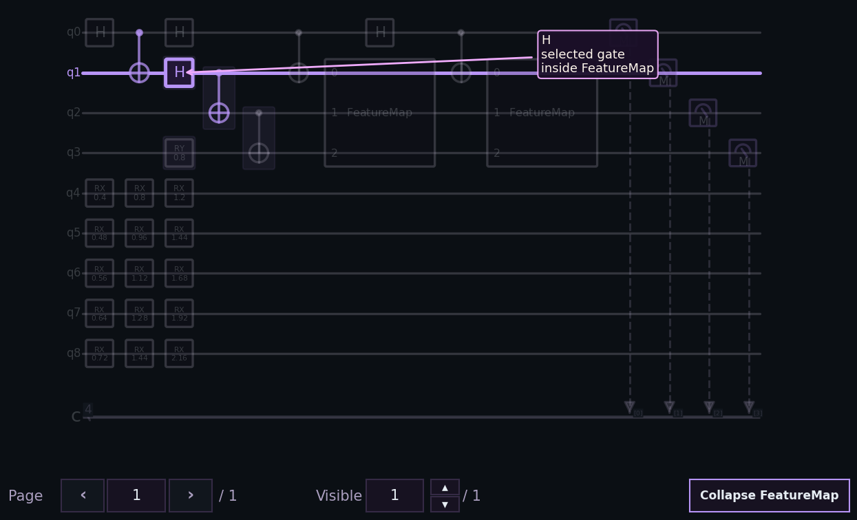
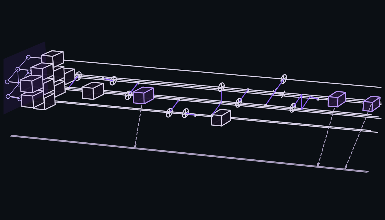
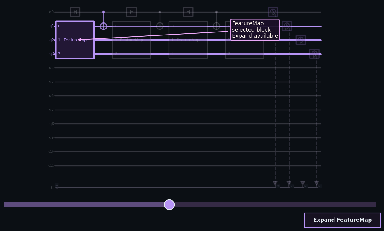
Visual Gallery
The library renders normal static images, managed exploration views, 3D topology scenes, and result distributions with the same public API shape.
| Static 2D circuit | Managed 2D exploration | 3D topology view |
|---|---|---|
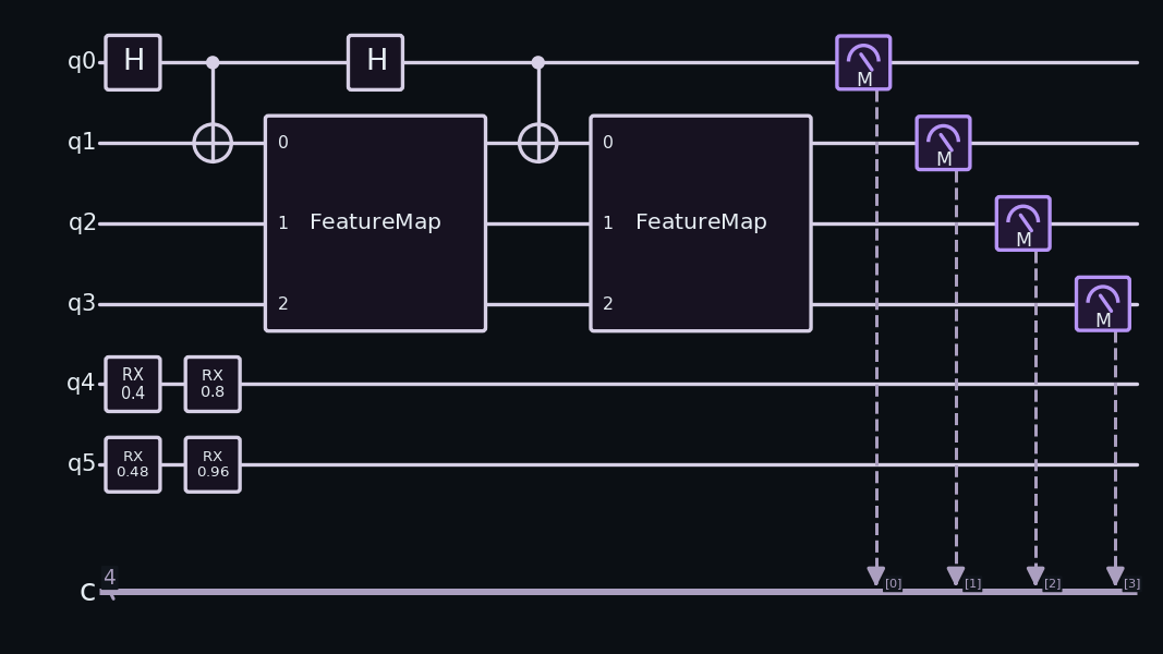 |
 |
 |
 |
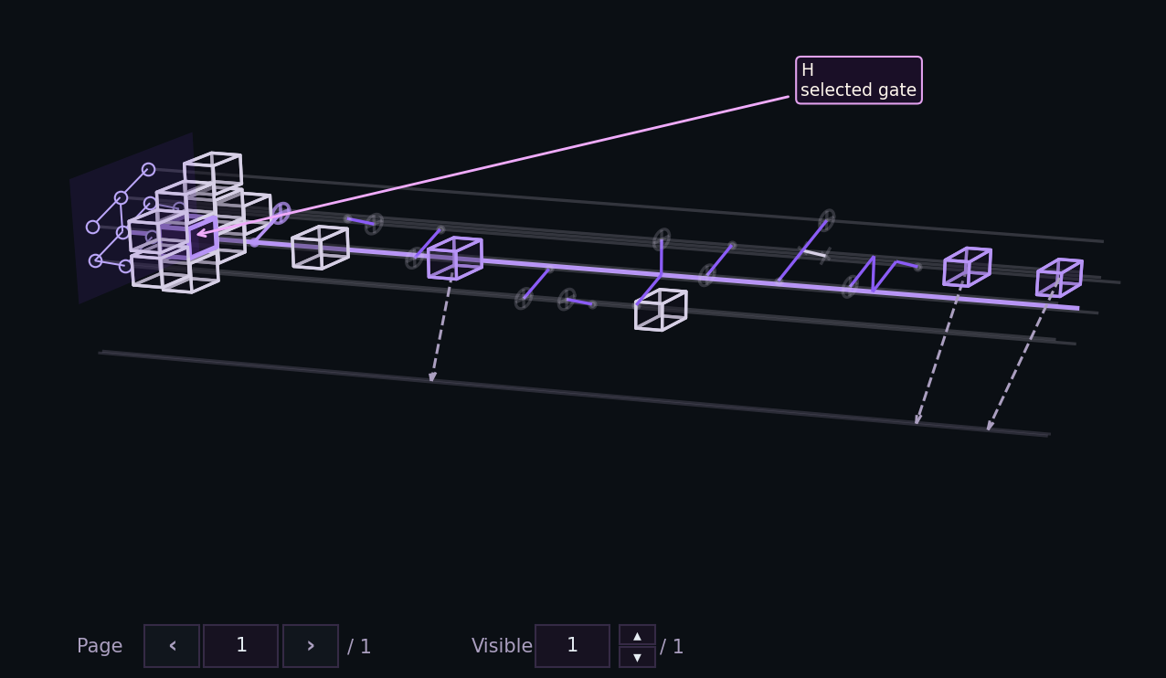 |
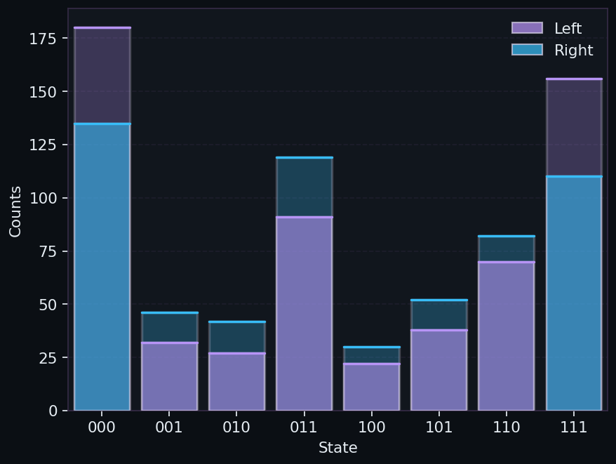 |
Install
Inside your local .venv:
The core package supports Python 3.11, 3.12, and 3.13. Optional framework extras
can have narrower platform support depending on their upstream packages.
The base install declares Matplotlib 3.8+ and NumPy 1.26+; optional extras
currently use Qiskit 2.0+, Cirq Core 1.6+, PennyLane 0.42+, MyQLM 1.11+,
CUDA-Q 0.14+ on Linux, and ipympl 0.10+.
Windows PowerShell:
.\.venv\Scripts\python.exe -m pip install quantum-circuit-drawer
Linux or WSL:
.venv/bin/python -m pip install quantum-circuit-drawer
If you only need saved images, that install is enough. If you also want interactive Matplotlib windows inside WSL2, pip install is not always enough on its own because Linux distributions often ship Tk as a separate system package. On Ubuntu or Debian under WSL2, install it once with:
sudo apt install python3-tk
Then verify GUI support from the same virtual environment:
.venv/bin/python -m tkinter
If that test window does not open, keep using show=False or output_path=... and check Troubleshooting.
Install only the extras you need:
Windows PowerShell:
.\.venv\Scripts\python.exe -m pip install "quantum-circuit-drawer[qiskit]"
.\.venv\Scripts\python.exe -m pip install "quantum-circuit-drawer[qasm3]"
.\.venv\Scripts\python.exe -m pip install "quantum-circuit-drawer[cirq]"
.\.venv\Scripts\python.exe -m pip install "quantum-circuit-drawer[pennylane]"
.\.venv\Scripts\python.exe -m pip install "quantum-circuit-drawer[myqlm]"
.\.venv\Scripts\python.exe -m pip install "quantum-circuit-drawer[notebook]"
Linux or WSL:
.venv/bin/python -m pip install "quantum-circuit-drawer[qiskit]"
.venv/bin/python -m pip install "quantum-circuit-drawer[qasm3]"
.venv/bin/python -m pip install "quantum-circuit-drawer[cirq]"
.venv/bin/python -m pip install "quantum-circuit-drawer[pennylane]"
.venv/bin/python -m pip install "quantum-circuit-drawer[myqlm]"
.venv/bin/python -m pip install "quantum-circuit-drawer[notebook]"
CUDA-Q is Linux/WSL2-only because the upstream package is not available for native Windows:
.venv/bin/python -m pip install "quantum-circuit-drawer[cudaq]"
Use the notebook extra when you want Jupyter hover, managed circuit controls, or interactive histograms with %matplotlib widget. It installs ipympl without making notebook tooling part of the base package.
Support matrix
This is the production support contract for the current release.
| Input path | Support level | Platform notes |
|---|---|---|
| Internal IR | Strong support | Core built-in path on Windows and Linux |
| Qiskit | Strong support | Primary external backend on Windows and Linux |
OpenQASM 2 text and .qasm files |
Strong support through the Qiskit extra | Install quantum-circuit-drawer[qiskit]; works on Windows and Linux |
OpenQASM 3 text and .qasm3 files |
Strong support through Qiskit plus qiskit-qasm3-import |
Install quantum-circuit-drawer[qasm3]; works on Windows and Linux when Qiskit's importer is available |
| Cirq | Best-effort on native Windows | Accepts cirq.Circuit and cirq.FrozenCircuit; prefer Linux or WSL for the most reliable repeated runs |
| PennyLane | Best-effort on native Windows | Prefer Linux or WSL for the most reliable repeated runs |
| MyQLM | Scoped adapter + contract support | Accepts qat.core.Circuit, Program, and QRoutine; adapter contract is covered, but it is not a first-class multiplatform CI backend |
| CUDA-Q | Linux/WSL2 only | Supports closed kernels plus scalar cudaq_args for runtime-argument kernels; upstream CUDA-Q is not available for native Windows |
Choose Your First Task
| If you want to... | Start here |
|---|---|
| Inspect a circuit before rendering | Analyze a circuit |
| Draw a circuit from a supported framework | Draw one circuit |
Draw OpenQASM 2/3 text or a .qasm / .qasm3 file |
Draw OpenQASM |
| Generate images from your terminal | Command line |
| Save a render from a script without opening a window | Save directly to a file |
| Export LaTeX for papers or notes | Export a circuit to LaTeX |
| Plot counts or probabilities | Plot one histogram |
| Compare circuit versions | Compare circuits |
| Compare distributions | Compare histograms |
| Build a circuit without a framework dependency | Build with public IR tools |
| Learn the full user-facing feature set | Extended guide |
| Explore framework-specific demos | Recommended demos |
Command Line
The package installs a small qcd command for the common "make me an image" workflow. It saves files without opening Matplotlib windows by default; add --show when you also want a window.
Windows PowerShell:
qcd draw bell.qasm --output bell.png --view 3d
qcd histogram counts.json --output counts.png
Linux or WSL:
qcd draw bell.qasm --output bell.png --view 3d
qcd histogram counts.json --output counts.png
qcd draw accepts OpenQASM text or .qasm / .qasm3 files. qcd histogram accepts JSON mappings such as {"00": 10, "11": 6} and can select nested payloads with --data-key counts.
Draw One Circuit
from qiskit import QuantumCircuit

from quantum_circuit_drawer import draw_quantum_circuit

circuit = QuantumCircuit(2, 1)
circuit.h(0)
circuit.cx(0, 1)
circuit.measure(1, 0)

result = draw_quantum_circuit(circuit, show=False)

figure = result.primary_figure
axes = result.primary_axes
This same shape works for the supported framework objects and for the public IR types.
For text styling, the default circuit style now uses use_mathtext="auto". That keeps
visible labels such as wire names and gate names in plain text by default, while still
using MathText automatically for parameter subtitles when it improves symbolic notation
such as theta, phi, or pi/2.
Analyze A Circuit Without Rendering
Use analyze_quantum_circuit(...) when you want a quick summary before opening windows or saving images:
from quantum_circuit_drawer import analyze_quantum_circuit

analysis = analyze_quantum_circuit(circuit)

summary = analysis.to_dict()
The analysis path prepares the same normalized circuit pipeline as drawing, but it does not render, call show(), or save output_path.
All public result objects also support post-render export helpers. Circuit results can call result.save("circuit.png"), result.save_all_pages("pages"), and result.to_dict(). Histogram results can also call result.to_csv("histogram.csv").
Draw OpenQASM
OpenQASM input uses Qiskit as the parser. Install the Qiskit extra for OpenQASM 2, and install the qasm3 extra when you want OpenQASM 3 support:
.\.venv\Scripts\python.exe -m pip install "quantum-circuit-drawer[qiskit]"
.\.venv\Scripts\python.exe -m pip install "quantum-circuit-drawer[qasm3]"
You can pass OpenQASM 2 or OpenQASM 3 text directly:
from quantum_circuit_drawer import draw_quantum_circuit

qasm = """
OPENQASM 2.0;
include "qelib1.inc";
qreg q[2];
creg c[1];
h q[0];
cx q[0],q[1];
measure q[1] -> c[0];
"""

result = draw_quantum_circuit(qasm, show=False)
Or draw a .qasm / .qasm3 file directly. framework="qasm" is optional when the path ends in .qasm or .qasm3, but it is useful when you want to be explicit:
from pathlib import Path

from quantum_circuit_drawer import draw_quantum_circuit

result = draw_quantum_circuit(
    Path("bell.qasm"),
    framework="qasm",
    show=False,
)
Draw CUDA-Q With Runtime Arguments
CUDA-Q is Linux/WSL2-only because the upstream package is not available for native Windows. Closed kernels work directly; kernels that take scalar runtime arguments use adapter_options={"cudaq_args": (...)}:
import cudaq

from quantum_circuit_drawer import (
    CircuitRenderOptions,
    DrawConfig,
    DrawSideConfig,
    draw_quantum_circuit,
)

kernel, size, theta = cudaq.make_kernel(int, float)
qubits = kernel.qalloc(size)
kernel.rx(theta, qubits[0])
kernel.mz(qubits)

result = draw_quantum_circuit(
    kernel,
    framework="cudaq",
    show=False,
    config=DrawConfig(
        side=DrawSideConfig(
            render=CircuitRenderOptions(
                adapter_options={"cudaq_args": (3, 0.25)},
            )
        ),
    ),
)
Save Directly To A File
from qiskit import QuantumCircuit

from quantum_circuit_drawer import draw_quantum_circuit

circuit = QuantumCircuit(2, 1)
circuit.h(0)
circuit.cx(0, 1)
circuit.measure(1, 0)

draw_quantum_circuit(
    circuit,
    output_path="bell.png",
    show=False,
)
This is the most common script workflow when you want a deterministic export without opening a GUI window.
Export A Circuit To LaTeX
Use circuit_to_latex(...) when you want the same circuit as source text instead of a Matplotlib figure:
from quantum_circuit_drawer import DrawMode, LatexBackend, circuit_to_latex

latex_result = circuit_to_latex(
    circuit,
    backend=LatexBackend.QUANTIKZ,
    mode=DrawMode.PAGES,
)

print(latex_result.source)
This is useful for papers, lecture notes, or slide decks where you want to keep editing the diagram on the LaTeX side.
Plot One Histogram
Counts
from quantum_circuit_drawer import (
    HistogramAppearanceOptions,
    HistogramConfig,
    plot_histogram,
)

result = plot_histogram(
    {"000": 51, "001": 14, "010": 9, "111": 49},
    sort="value_desc",
    top_k=3,
    show=False,
    config=HistogramConfig(
        appearance=HistogramAppearanceOptions(show_uniform_reference=True),
    ),
)
Quasi-probabilities
from quantum_circuit_drawer import (
    HistogramAppearanceOptions,
    HistogramConfig,
    plot_histogram,
)

result = plot_histogram(
    {0: 0.52, 3: -0.08, 4: 0.17, 7: 0.39},
    kind="quasi",
    show=False,
    config=HistogramConfig(
        appearance=HistogramAppearanceOptions(
            draw_style="soft",
            show_uniform_reference=True,
        ),
    ),
)
Joint marginal on selected qubits
from quantum_circuit_drawer import plot_histogram

result = plot_histogram(
    {"101": 2, "001": 1, "111": 3},
    qubits=(0, 2),
    show=False,
)
qubits=(0, 2) keeps the requested order, so the marginal labels are built as q0 followed by q2.
Compare Two Or More Circuits
from qiskit import QuantumCircuit, transpile

from quantum_circuit_drawer import compare_circuits

source = QuantumCircuit(3, 3)
source.h(0)
source.cx(0, 1)
source.cx(1, 2)
source.measure(range(3), range(3))

transpiled = transpile(source, basis_gates=["u", "cx"], optimization_level=2)

result = compare_circuits(
    source,
    transpiled,
    left_title="Original",
    right_title="Transpiled",
    show=False,
)
CircuitCompareResult gives you:
- a compact summary figure by default
- one
DrawResultper circuit, with each circuit rendered in its own normalpages_controlsfigure unless you requestmode="full"or pass caller-owned axes - structural metrics such as operation counts, measurement counts, swap counts, and differing layers
For three or more circuits, pass the extra circuits as positional arguments and provide titles=(...). The summary table switches from a two-side delta column to one column per circuit; lower aggregate counts are highlighted in green and higher aggregate counts in red for each row.
Compare Two Or More Histograms
from quantum_circuit_drawer import compare_histograms

ideal = {"00": 0.5, "11": 0.5}
sampled = {"00": 473, "01": 19, "10": 24, "11": 484}

result = compare_histograms(
    ideal,
    sampled,
    sort="delta_desc",
    left_label="Ideal",
    right_label="Sampled",
    show=False,
)
This is useful when you want one aligned state space and quick metrics such as total variation distance. On interactive Matplotlib backends, the compare legend is clickable so you can focus one selected series at a time while keeping the axes and hover state in sync.
For three or more distributions, pass extra data objects after the first two and set series_labels=(...). Sorting with sort="delta_desc" uses the largest spread across all visible series.
Build With Public IR Tools
If you do not want to depend on a framework, you can build directly with the public IR tools or use CircuitBuilder.
CircuitBuilder
from quantum_circuit_drawer import CircuitBuilder, draw_quantum_circuit

circuit = (
    CircuitBuilder(2, 1, name="builder_demo")
    .h(0)
    .cx(0, 1)
    .measure(1, 0)
    .build()
)

draw_quantum_circuit(circuit, show=False)
Raw CircuitIR
If you need complete control over wires, operations, and metadata, use the public quantum_circuit_drawer.ir types directly. The best minimal example for that path is the bundled ir-basic-workflow demo.
Modes, Hover, And 3D
The most common choices are:
DrawMode.AUTO: notebook ->pages, normal script ->pages_controlsDrawMode.PAGES: easiest for notebook display and export-oriented flowsDrawMode.PAGES_CONTROLS: best default for normal scriptsDrawMode.SLIDER: best when you want a viewport through a wide circuitDrawMode.FULL: best when the circuit fits comfortably in one scene
Managed pages_controls and slider figures now enable keyboard navigation and block toggling by default. That includes arrows, Home / End, PageUp / PageDown, Tab / Shift+Tab, Esc, 0, ?, and +/- where the mode supports them. In pages_controls, Up grows the visible page stack, Down shrinks it, and Tab / Shift+Tab move column by column even when that means stepping to the next or previous page. Use CircuitRenderOptions(keyboard_shortcuts=False, double_click_toggle=False) if you want to turn those interactions off.
Example:
from quantum_circuit_drawer import (
    CircuitAppearanceOptions,
    CircuitRenderOptions,
    DrawConfig,
    DrawMode,
    DrawSideConfig,
    OutputOptions,
    draw_quantum_circuit,
)

result = draw_quantum_circuit(
    circuit,
    config=DrawConfig(
        side=DrawSideConfig(
            render=CircuitRenderOptions(mode=DrawMode.PAGES_CONTROLS),
            appearance=CircuitAppearanceOptions(
                hover={"enabled": True, "show_size": True},
            ),
        ),
        output=OutputOptions(show=False),
    ),
)
For 3D:
from quantum_circuit_drawer import (
    CircuitRenderOptions,
    DrawConfig,
    DrawMode,
    DrawSideConfig,
    OutputOptions,
    draw_quantum_circuit,
)

result = draw_quantum_circuit(
    circuit,
    config=DrawConfig(
        side=DrawSideConfig(
            render=CircuitRenderOptions(
                view="3d",
                mode=DrawMode.PAGES_CONTROLS,
                topology="grid",
                topology_qubits="used",
                topology_resize="error",
                topology_menu=True,
            ),
        ),
        output=OutputOptions(show=False),
    ),
)
The built-in 3D topologies ("line", "grid", "star", "star_tree", and "honeycomb") are flexible builders, so they can be used with arbitrary positive qubit counts. The "honeycomb" builder uses an IBM-inspired compact hexagonal footprint. For real Qiskit devices, build a static topology with HardwareTopology.from_qiskit_backend(backend). If a topology has more physical nodes than the circuit uses, topology_qubits="used" shows only the allocated nodes while topology_qubits="all" shows the full hardware footprint. If a functional or periodic topology is too small, topology_resize="fit" rebuilds it for the circuit size; static HardwareTopology instances stay fixed and raise a clear error when they are too small.
If you want to see the managed 2D controls intentionally exercised instead of configuring them from scratch, start with qiskit-2d-exploration-showcase.
If you want the same style of managed exploration in 3D, start with qiskit-3d-exploration-showcase.
Recommended Demos
The fastest way to see the current strengths of the library is to run one of the bundled showcase demos:
| Demo id | What it highlights |
|---|---|
qiskit-2d-exploration-showcase |
Managed 2D exploration with Wires: All/Active, Ancillas: Show/Hide, folded-wire markers, and contextual Collapse / Expand |
qiskit-3d-exploration-showcase |
Managed 3D exploration with topology-aware selection, persistent expanded-block highlights, and contextual Collapse / Expand |
qiskit-control-flow-showcase |
Expanded Qiskit control-flow frames, visible switch summaries, and open controls |
qiskit-composite-modes-showcase |
Compact versus expanded composite instructions on the same workflow |
openqasm-showcase |
OpenQASM text input through the Qiskit parser path |
ir-basic-workflow |
Framework-free rendering from the public CircuitIR types |
public-api-utilities-showcase |
Analysis, result metadata, page exports, histogram CSV export, and circuit_to_latex(...) |
caller-managed-axes-showcase |
Circuit, histogram, and comparison rendering on caller-managed axes |
style-accessible-showcase |
Accessible circuit and histogram styling |
diagnostics-showcase |
Diagnostics, warnings, and resolved-mode metadata |
cli-export-showcase |
Terminal-oriented qcd JSON histogram export |
qiskit-backend-topology-showcase |
Qiskit backend topology conversion into a 3D hardware view |
cirq-native-controls-showcase |
Cirq native controls, classical conditions, and CircuitOperation provenance |
pennylane-terminal-outputs-showcase |
PennyLane mid-measurement, qml.cond(...), plus terminal output boxes |
myqlm-structural-showcase |
Compact composite routines on the native MyQLM adapter path |
cudaq-kernel-showcase |
The supported CUDA-Q subset with scalar runtime arguments, reset, basis measurements, and static control summaries |
compare-circuits-multi-transpile |
One Qiskit source circuit compared with several transpilation optimization levels |
compare-histograms-ideal-vs-sampled |
A lightweight comparison workflow with no framework extra required, including clickable legend toggles on interactive backends |
compare-histograms-multi-series |
A multi-series overlay for ideal, noisy, raw hardware, and mitigated distributions |
histogram-quasi-nonnegative |
A compact histogram demo for non-negative quasi-probabilities that keep the vertical axis anchored at zero |
In the examples catalog, each showcase has both a direct script filename such as examples/qiskit_2d_exploration_showcase.py and, when you use the shared runners, a matching demo_id such as qiskit-2d-exploration-showcase.
If you are running the bundled examples from this repository rather than installing the published package, install the optional extras you need inside your local .venv, for example .\.venv\Scripts\python.exe -m pip install -e ".[qiskit]" on Windows PowerShell or .venv/bin/python -m pip install -e ".[qiskit]" on Linux or WSL.
Windows PowerShell:
.\.venv\Scripts\python.exe examples\qiskit_2d_exploration_showcase.py
.\.venv\Scripts\python.exe examples\qiskit_3d_exploration_showcase.py
.\.venv\Scripts\python.exe examples\qiskit_control_flow_showcase.py
.\.venv\Scripts\python.exe examples\qiskit_composite_modes_showcase.py --composite-mode expand
.\.venv\Scripts\python.exe examples\openqasm_showcase.py
.\.venv\Scripts\python.exe examples\ir_basic_workflow.py
.\.venv\Scripts\python.exe examples\public_api_utilities_showcase.py
.\.venv\Scripts\python.exe examples\caller_managed_axes_showcase.py
.\.venv\Scripts\python.exe examples\style_accessible_showcase.py
.\.venv\Scripts\python.exe examples\diagnostics_showcase.py
.\.venv\Scripts\python.exe examples\cli_export_showcase.py
.\.venv\Scripts\python.exe examples\qiskit_backend_topology_showcase.py
.\.venv\Scripts\python.exe examples\compare_circuits_multi_transpile.py
.\.venv\Scripts\python.exe examples\compare_histograms_ideal_vs_sampled.py
.\.venv\Scripts\python.exe examples\compare_histograms_multi_series.py
.\.venv\Scripts\python.exe examples\histogram_quasi_nonnegative.py
Linux or WSL:
.venv/bin/python examples/qiskit_2d_exploration_showcase.py
.venv/bin/python examples/qiskit_3d_exploration_showcase.py
.venv/bin/python examples/qiskit_control_flow_showcase.py
.venv/bin/python examples/qiskit_composite_modes_showcase.py --composite-mode expand
.venv/bin/python examples/openqasm_showcase.py
.venv/bin/python examples/ir_basic_workflow.py
.venv/bin/python examples/public_api_utilities_showcase.py
.venv/bin/python examples/caller_managed_axes_showcase.py
.venv/bin/python examples/style_accessible_showcase.py
.venv/bin/python examples/diagnostics_showcase.py
.venv/bin/python examples/cli_export_showcase.py
.venv/bin/python examples/qiskit_backend_topology_showcase.py
.venv/bin/python examples/compare_circuits_multi_transpile.py
.venv/bin/python examples/compare_histograms_ideal_vs_sampled.py
.venv/bin/python examples/compare_histograms_multi_series.py
.venv/bin/python examples/histogram_quasi_nonnegative.py
The CLI export showcase writes examples/output/cli-export-showcase.png by default. Use --output to choose another PNG path.
The full curated catalog, including the mapping between runner demo_id values and direct script filenames, lives in examples/README.md.
Documentation
Use these pages depending on what you need:
Release history Release notifications | RSS feed


Download files
Download the file for your platform. If you're not sure which to choose, learn more about installing packages.
Source Distribution
Built Distribution
Filter files by name, interpreter, ABI, and platform.
If you're not sure about the file name format, learn more about wheel file names.
Copy a direct link to the current filters
File details
Details for the file quantum_circuit_drawer-1.1.0.tar.gz.
File metadata
- Download URL: quantum_circuit_drawer-1.1.0.tar.gz
- Upload date:
- Size: 354.8 kB
- Tags: Source
- Uploaded using Trusted Publishing? No
- Uploaded via: twine/6.2.0 CPython/3.12.10
File hashes
| Algorithm | Hash digest | |
|---|---|---|
| SHA256 |
53681e636d8f0464b5ef2aefd0d6cc0444cacf6788582c81b2285e0b3f8d320b
|
|
| MD5 |
92e40d7d005de54ec496dae64a09cdb8
|
|
| BLAKE2b-256 |
ec6545a088e6babf69e632792d4bebca90170ffcc676fd47ae6acc8e917e13a7
|
File details
Details for the file quantum_circuit_drawer-1.1.0-py3-none-any.whl.
File metadata
- Download URL: quantum_circuit_drawer-1.1.0-py3-none-any.whl
- Upload date:
- Size: 418.5 kB
- Tags: Python 3
- Uploaded using Trusted Publishing? No
- Uploaded via: twine/6.2.0 CPython/3.12.10
File hashes
| Algorithm | Hash digest | |
|---|---|---|
| SHA256 |
29e634e9196cd7f4122b84cced4300b7c05041b66f0a5e68d646d1ca0a25bd62
|
|
| MD5 |
b8a3ea7eff5892cd11cf234dc89e9244
|
|
| BLAKE2b-256 |
7195b6b44a22f45d4da6dbf4343a5d6fc4476c7b9704251edf10de3ad4a3a193
|


