










radioactivedecay is a Python package for radioactive decay calculations.
It supports decay chains of radionuclides, metastable states and branching
decays. By default it uses the decay data from ICRP Publication 107, which
contains 1252 radionuclides of 97 elements, and atomic mass data from the
Atomic Mass Data Center.
The code solves the radioactive decay differential equations analytically using NumPy and SciPy linear algebra routines. There is also a high numerical precision calculation mode employing SymPy routines. This gives more accurate results for decay chains containing radionuclides with orders of magnitude differences between the half-lives.
This is free-to-use open source software. It was created for engineers, technicians and researchers who work with radioactivity, and for educational use.
- Full Documentation: https://radioactivedecay.github.io/
Installation
radioactivedecay requires Python 3.9+. Install radioactivedecay from
the Python Package Index using
pip:
$ pip install radioactivedecay
or from conda-forge:
$ conda install -c conda-forge radioactivedecay
Either command will attempt to install the dependencies (Matplotlib, NetworkX, NumPy, Pandas, SciPy, Setuptools & SymPy) if they are not already present in the environment.
Usage
Decay calculations
Create an Inventory of radionuclides and decay it as follows:
>>> import radioactivedecay as rd
>>> Mo99_t0 = rd.Inventory({'Mo-99': 2.0}, 'Bq')
>>> Mo99_t1 = Mo99_t0.decay(20.0, 'h')
>>> Mo99_t1.activities('Bq')
{'Mo-99': 1.6207863893776937, 'Ru-99': 0.0,
 'Tc-99': 9.05304236308454e-09, 'Tc-99m': 1.3719829376710406}
An Inventory of 2.0 Bq of Mo-99 was decayed for 20 hours, producing the
radioactive progeny Tc-99m and Tc-99, and the stable nuclide Ru-99.
We supplied 'h' as an argument to decay() to specify the decay time
period had units of hours. Supported time units include 'μs', 'ms',
's', 'm', 'h', 'd', 'y' etc. Note seconds ('s') is the
default if no unit is supplied to decay().
Use cumulative_decays() to calculate the total number of atoms of each
radionuclide that decay over the decay time period:
>>> Mo99_t0.cumulative_decays(20.0, 'h')
{'Mo-99': 129870.3165339939, 'Tc-99m': 71074.31925850797,
'Tc-99': 0.0002724635511147602}
Radionuclides can be specified in four equivalent ways in radioactivedecay:
three variations of nuclide strings or by
canonical ids. For example, the
following are equivalent ways of specifying 222Rn and
192nIr:
'Rn-222','Rn222','222Rn',862220000,'Ir-192n','Ir192n','192nIr',771920002.
Inventories can be created by supplying activity ('Bq', 'Ci',
'dpm'...), mass ('g', 'kg'...), mole ('mol', 'kmol'...)
units, or numbers of nuclei ('num') to the Inventory() constructor. Use
the methods activities(), masses(), moles(), numbers(),
activity_fractions(), mass_fractions() and mole_fractions() to
obtain the contents of the inventory in different formats:
>>> H3_t0 = rd.Inventory({'H-3': 3.0}, 'g')
>>> H3_t1 = H3_t0.decay(12.32, 'y')
>>> H3_t1.masses('g')
{'H-3': 1.5, 'He-3': 1.4999900734297729}
>>> H3_t1.mass_fractions()
{'H-3': 0.5000016544338455, 'He-3': 0.4999983455661545}

>>> C14_t0 = rd.Inventory({'C-14': 3.2E24}, 'num')
>>> C14_t1 = C14_t0.decay(3000, 'y')
>>> C14_t1.moles('mol')
{'C-14': 3.6894551567795797, 'N-14': 1.6242698581767292}
>>> C14_t1.mole_fractions()
{'C-14': 0.6943255713073281, 'N-14': 0.3056744286926719}
Plotting decay graphs
Use the plot() method to graph of the decay of an inventory over time:
>>> Mo99_t0.plot(20, 'd', yunits='Bq')
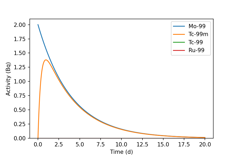
The graph shows the decay of Mo-99 over 20 days, leading to the ingrowth of Tc-99m and a trace quantity of Tc-99. The activity of Ru-99 is strictly zero as it is the stable nuclide at the end of the decay chain. Graphs are drawn using Matplotlib.
Fetching decay data
The Nuclide class can be used to fetch decay information for
individual radionuclides, e.g. for Rn-222:
>>> nuc = rd.Nuclide('Rn-222')
>>> nuc.half_life('s')
330350.4
>>> nuc.half_life('readable')
'3.8235 d'
>>> nuc.progeny()
['Po-218']
>>> nuc.branching_fractions()
[1.0]
>>> nuc.decay_modes()
['α']
>>> nuc.Z  # proton number
86
>>> nuc.A  # nucleon number
222
>>> nuc.atomic_mass  # atomic mass in g/mol
222.01757601699998
There are similar inventory methods for fetching decay data:
>>> Mo99_t1.half_lives('readable')
{'Mo-99': '65.94 h', 'Ru-99': 'stable', 'Tc-99': '0.2111 My', 'Tc-99m': '6.015 h'}
>>> Mo99_t1.progeny()
{'Mo-99': ['Tc-99m', 'Tc-99'], 'Ru-99': [], 'Tc-99': ['Ru-99'], 'Tc-99m': ['Tc-99', 'Ru-99']}
>>> Mo99_t1.branching_fractions()
{'Mo-99': [0.8773, 0.1227], 'Ru-99': [], 'Tc-99': [1.0], 'Tc-99m': [0.99996, 3.7e-05]}
>>> Mo99_t1.decay_modes()
{'Mo-99': ['β-', 'β-'], 'Ru-99': [], 'Tc-99': ['β-'], 'Tc-99m': ['IT', 'β-']}
Decay chain diagrams
The Nuclide class includes a plot() method for drawing decay chain
diagrams:
>>> nuc = rd.Nuclide('Mo-99')
>>> nuc.plot()
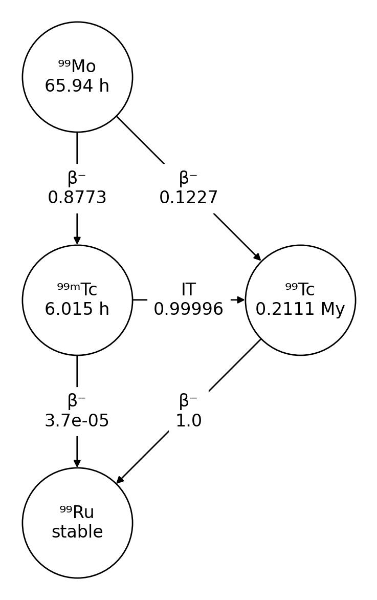
These diagrams are drawn using NetworkX and Matplotlib.
High numerical precision decay calculations
radioactivedecay includes an InventoryHP class for high numerical
precision calculations. This class can give more reliable decay calculation
results for chains containing long- and short-lived radionuclides:
>>> U238_t0 = rd.InventoryHP({'U-238': 1.0})
>>> U238_t1 = U238_t0.decay(10.0, 'd')
>>> U238_t1.activities()
{'At-218': 1.4511675857141352e-25,
 'Bi-210': 1.8093327888942224e-26,
 'Bi-214': 7.09819414496093e-22,
 'Hg-206': 1.9873081129046843e-33,
 'Pa-234': 0.00038581180879502017,
 'Pa-234m': 0.24992285949158477,
 'Pb-206': 0.0,
 'Pb-210': 1.0508864357335218e-25,
 'Pb-214': 7.163682655782086e-22,
 'Po-210': 1.171277829871092e-28,
 'Po-214': 7.096704966148592e-22,
 'Po-218': 7.255923469955255e-22,
 'Ra-226': 2.6127168262000313e-21,
 'Rn-218': 1.4511671865210924e-28,
 'Rn-222': 7.266530698712501e-22,
 'Th-230': 8.690585458641225e-16,
 'Th-234': 0.2499481473619856,
 'Tl-206': 2.579902288672889e-32,
 'Tl-210': 1.4897029111914831e-25,
 'U-234': 1.0119788393651999e-08,
 'U-238': 0.9999999999957525}
How radioactivedecay works
radioactivedecay calculates an analytical solution to the radioactive decay
differential equations using linear algebra operations. It implements the
method described in this paper:
M Amaku, PR Pascholati & VR Vanin, Comp. Phys. Comm. 181, 21-23
(2010). See the
theory docpage for more
details.
It uses NumPy and SciPy routines for standard decay calculations (double-precision floating-point operations), and SymPy for arbitrary numerical precision calculations.
By default radioactivedecay uses decay data from
ICRP Publication 107
(2008) and atomic mass
data from the Atomic Mass Data Center
(AMDC - AME2020 and Nubase2020 evaluations).
The datasets repo contains
Jupyter Notebooks for creating decay datasets that can be used by
radioactivedecay, e.g. ICRP
107.
The comparisons repo
contains some checks of radioactivedecay against
PyNE
and Radiological
Toolbox.
Tests
From the base directory run:
$ python -m unittest discover
License
radioactivedecay is open source software released under the MIT License.
See LICENSE
file for details.
The default decay data used by radioactivedecay (ICRP-107) is copyright
2008 A. Endo and K.F. Eckerman and distributed under a separate
license.
The default atomic mass data is from AMDC
(license).
Citation
If you find this package useful for your research, please consider citing the
paper on radioactivedecay published in the
Journal of Open Source Software:
Alex Malins & Thom Lemoine, radioactivedecay: A Python package for radioactive decay calculations. Journal of Open Source Software, 7 (71), 3318 (2022). DOI: 10.21105/joss.03318.
Contributing
Contributors are welcome to fix bugs, add new features or make feature requests. Please open an Issue, Pull Request or new Discussions thread at GitHub repository.
Please read the contribution guidelines.
1 maintainer

Metadata
1 maintainer
Release files for radioactivedecay 0.6.1
For a detailed explanation of source distributions (sdists) and built distributions (wheels), please see the package formats documentation.
Source distribution (sdist)
| File | Size | Uploaded | |
|---|---|---|---|
| radioactivedecay-0.6.1.tar.gz | 973.9 kB | Details |
Built distribution (wheel)
| File | Interpreter | ABI | Platform | Reset |
|---|---|---|---|---|
| radioactivedecay-0.6.1-py3-none-any.whl | Python 3 | none | any | Details |
Total release size: 1.9 MB
Release files / radioactivedecay-0.6.1.tar.gz
| Download URL | radioactivedecay-0.6.1.tar.gz |
|---|---|
| Size | 973.9 kB |
| Tags | Source |
|
SHA-256 checksum How to use checksums |
a5c32ffd397edbb829f959e7ce941ce95e9d8168b539853f1541ff02ddd603eb
|
|
BLAKE2b-256 checksum How to use checksums |
f3f2731f06a11b3ee200f1634358c987f877e743e0d16a3a279262ca00227c90
|
| Upload date | |
|
Uploaded using Trusted Publishing? What is trusted publishing? |
No |
| Uploaded via |
twine/6.0.1 CPython/3.13.1
|
Release files / radioactivedecay-0.6.1-py3-none-any.whl
| Download URL | radioactivedecay-0.6.1-py3-none-any.whl |
|---|---|
| Size | 955.6 kB |
| Tags | Python 3 |
|
SHA-256 checksum How to use checksums |
b0eec1e57ba62154220585dd04bd4a41a5c031d3e2bef5ebeaff798a51fa8465
|
|
BLAKE2b-256 checksum How to use checksums |
5be944f69eea326c2df4b5a7bd0dedf3cb1da283c868d66050f7ff9ce109289d
|
| Upload date | |
|
Uploaded using Trusted Publishing? What is trusted publishing? |
No |
| Uploaded via |
twine/6.0.1 CPython/3.13.1
|














