

Reno System Dynamics (reno-sd)






Reno is a tool for creating, visualizing, and analyzing system dynamics models in Python. It additionally has the ability to convert models to PyMC, allowing Bayesian inference on models with variables that include prior probability distributions.
Reno models are created by defining the equations for the various stocks, flows,
and variables, and can then be simulated over time similar to something like
Insight Maker, examples of which can be seen below
and in the notebooks folder.
Currently, models only support discrete timesteps (technically implementing difference equations rather than true differential equations.)
Installation
Install from PyPI via:
pip install reno-sd
Install from conda-forge with:
conda install reno-sd
Example
A classic system dynamics example is the predator-prey population model, described by the Lotka-Volterra equations.
Implementing these in Reno would look something like:
import reno

predator_prey = reno.Model(name="predator_prey", steps=200, doc="Classic predator-prey interaction model example")

with predator_prey:
    # make stocks to monitor the predator/prey populations over time
    rabbits = reno.Stock(init=100.0)
    foxes = reno.Stock(init=100.0)

    # free variables that can quickly be changed to influence equilibrium
    rabbit_growth_rate = reno.Variable(.1, doc="Alpha")
    rabbit_death_rate = reno.Variable(.001, doc="Beta")
    fox_death_rate = reno.Variable(.1, doc="Gamma")
    fox_growth_rate = reno.Variable(.001, doc="Delta")

    # flows that define how much the stocks change in a timestep
    rabbit_births = reno.Flow(rabbit_growth_rate * rabbits)
    rabbit_deaths = reno.Flow(rabbit_death_rate * rabbits * foxes, max=rabbits)
    fox_deaths = reno.Flow(fox_death_rate * foxes, max=foxes)
    fox_births = reno.Flow(fox_growth_rate * rabbits * foxes)

    # hook up inflows/outflows for stocks
    rabbit_births >> rabbits >> rabbit_deaths
    fox_births >> foxes >> fox_deaths
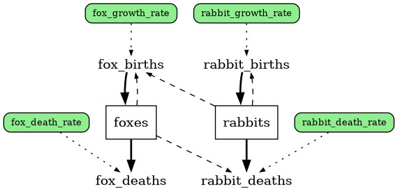
The stock and flow diagram for this model (obtainable via predator_prey.graph()) looks
like this: (green boxes are variables, white boxes are stocks, the labels between
arrows are the flows)
Once a model is defined it can be called like a function, optionally configuring
any free variables/initial values by passing them as arguments. You can print the
output of predator_prey.get_docs() to see a docstring showing all possible arguments and
what calling it should look like:
>>> print(predator_prey.get_docs())
Classic predator-prey interaction model example

Example:
	predator_prey(rabbit_growth_rate=0.1, rabbit_death_rate=0.001, fox_death_rate=0.1, fox_growth_rate=0.001, rabbits_0=100.0, foxes_0=100.0)

Args:
	rabbit_growth_rate: Alpha
	rabbit_death_rate: Beta
	fox_death_rate: Gamma
	fox_growth_rate: Delta
	rabbits_0
	foxes_0
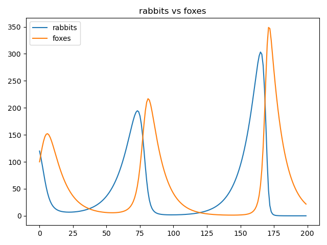
To run and plot the population stocks:
predator_prey(fox_growth_rate=.002, rabbit_death_rate=.002, rabbits_0=120.0)
reno.plot_refs([(predator_prey.rabbits, predator_prey.foxes)])
To use Bayesian inference, we define one or more metrics that can be observed (can
have defined likelihoods.) For instance, we could determine what rabbit population
growth rate would need to be for the fox population to oscillate somewhere between
20-120. Transpiling into PyMC and running the inference process is similar to the
normal model call, but with .pymc(), specifying any free variables (at least
one will need to be defined as a prior probability distribution), observations
to target, and any sampling/pymc parameters:
with predator_prey:
    minimum_foxes = reno.Metric(foxes.timeseries.series_min())
    maximum_foxes = reno.Metric(foxes.timeseries.series_max())

trace = predator_prey.pymc(
    n=1000,
    fox_growth_rate=reno.Normal(.001, .0001),  # specify some variables as distributions to sample from
    rabbit_growth_rate=reno.Normal(.1, .01),   # specify some variables as distributions to sample from
    observations=[
        reno.Observation(minimum_foxes, 5, [20]),  # likelihood normally distributed around 20 with SD of 5
        reno.Observation(maximum_foxes, 5, [120]), # likelihood normally distributed around 120 with SD of 5
    ]
)
To see the shift in prior versus posterior distributions, we can plot the random
variables and some of the relevant stocks using plot_trace_refs:
reno.plot_trace_refs(
    predator_prey,
    {"prior": trace.prior, "post": trace.posterior},
    ref_list=[
        predator_prey.minimum_foxes,
        predator_prey.maximum_foxes,
        predator_prey.fox_growth_rate,
        predator_prey.rabbit_growth_rate,
        predator_prey.foxes,
        predator_prey.rabbits
    ],
    figsize=(8, 5),
)
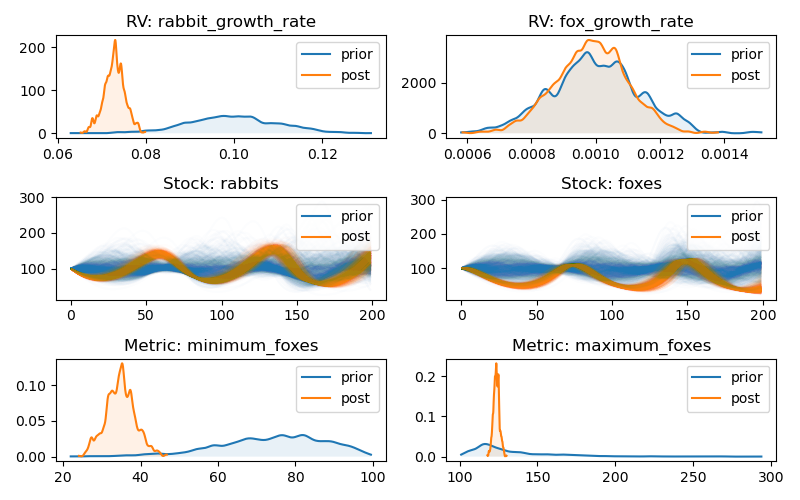
showing that the rabbit_growth_rate needs to be around 0.07 in order for
those observations to be met.
For a more in-depth introduction to reno, see the tub example in the ./notebooks folder.
Explorer UI
Reno comes with a browser-based graphical explorer, allowing you to load models and interactively test different configurations and Bayesian analysis runs. The explorer implements a customizable tab view, where each tab can be populated with configurable diagrams, plots, and text panels to describe interesting results. Overall sessions can be saved and reloaded later, and tabs can be downloaded as PDF documents for easier sharing.

To run the explorer, use the reno command. See command line arguments in the
documentation:
https://ornl.github.io/reno/stable/user/explorer.html
Documentation
For the API reference as well as (eventually) the user guide, see https://ornl.github.io/reno/stable
Citation
To cite usage of Reno, please use the following bibtex:
@misc{doecode_166929,
    title = {Reno},
    author = {Martindale, Nathan and Stomps, Jordan and Phathanapirom, Urairisa B.},
    abstractNote = {Reno is a tool for creating, visualizing, and analyzing system dynamics models in Python. It additionally has the ability to convert models to PyMC, allowing Bayesian inference on models with variables that include prior probability distributions.},
    doi = {10.11578/dc.20251015.1},
    url = {https://doi.org/10.11578/dc.20251015.1},
    howpublished = {[Computer Software] \url{https://doi.org/10.11578/dc.20251015.1}},
    year = {2025},
    month = {oct}
}
1 maintainer

Metadata
1 maintainer
Release files for reno-sd 0.15.1
For a detailed explanation of source distributions (sdists) and built distributions (wheels), please see the package formats documentation.
Source distribution (sdist)
| File | Size | Uploaded | |
|---|---|---|---|
| reno_sd-0.15.1.tar.gz | 159.9 kB | Details |
Built distribution (wheel)
| File | Interpreter | ABI | Platform | Reset |
|---|---|---|---|---|
| reno_sd-0.15.1-py3-none-any.whl | Python 3 | none | any | Details |
Total release size: 300.9 kB
Release files / reno_sd-0.15.1.tar.gz
| Download URL | reno_sd-0.15.1.tar.gz |
|---|---|
| Size | 159.9 kB |
| Tags | Source |
|
SHA-256 checksum How to use checksums |
cdf5c1bc3144e9c854ede4e64fefcde1d57232ae789203b85d3d866ba10c767e
|
|
BLAKE2b-256 checksum How to use checksums |
b17f9ebb1c41f71fd66640dbcd45ee582822b75deec8f8828f57bd9f6fb76b49
|
| Upload date | |
|
Uploaded using Trusted Publishing? What is trusted publishing? |
No |
| Uploaded via |
twine/6.2.0 CPython/3.12.12
|
Release files / reno_sd-0.15.1-py3-none-any.whl
| Download URL | reno_sd-0.15.1-py3-none-any.whl |
|---|---|
| Size | 141.0 kB |
| Tags | Python 3 |
|
SHA-256 checksum How to use checksums |
2fe539697fc848c0cab1df20be237da723dbb3ea3d24cb05188dacfb9d020e7a
|
|
BLAKE2b-256 checksum How to use checksums |
8ad18b48b67a607bb9db5a10935b7037480f28948f95b71e074035d2e214ef54
|
| Upload date | |
|
Uploaded using Trusted Publishing? What is trusted publishing? |
No |
| Uploaded via |
twine/6.2.0 CPython/3.12.12
|














