
rota-order




Rotational Order Tracking & Analysis. Rota is Latin for "wheel".
rota-order is a lightweight, open-source Python library for order analysis of noise and vibration signals from rotating machinery (engines, electric motors, gearboxes), with tools for order-based sound resynthesis. It depends only on NumPy and SciPy. The project rule is that each function is implemented independently from the published literature and tested on synthetic signals with known analytic ground truth.
The design document is ROADMAP.md.
Status
Pre-alpha. The current release is 0.8.0; functions and signatures may still change before 1.0.
| Module | Contents | Since |
|---|---|---|
rota_order.speed |
Tachometer pulses to rpm, rpm to shaft angle, control-signal cleanup and resampling, vehicle speed to rpm, steady-segment selection; tacholess speed estimation (order comb + dynamic programming, with confidence and search-boundary flags); virtual rpm; alignment of signals by GCC-PHAT delay and onset detection | 0.1–0.5 |
rota_order.angle |
Resampling from uniform time to uniform shaft angle (computed order tracking) with angle-domain anti-aliasing; the inverse mapping; time warping to a reference speed (stationarize) | 0.1, 0.3 |
rota_order.maps |
Rpm-frequency (Campbell) map, rpm-order map; binning of frames into rpm bins (per segment, minimum count, phase-coherent option) | 0.1, 0.5 |
rota_order.slices |
Order spectrum, order slice; frequency slice, overall level, any metric binned along rpm, attribution of frequency tracks to orders, order share | 0.1, 0.5 |
rota_order.extract |
Order extraction (second-generation Vold-Kalman filter, joint over orders and shafts; phase-locked tracked harmonics), order removal, residual, resolvability check | 0.2 |
rota_order.resynth |
Order tables (explicit peak/RMS), additive order synthesis offline and in blocks, broadband synthesis without frame-rate pumping, order editing, speed remapping, order-plus-residual recombination, steady listening excerpts, provenance sidecars | 0.3 |
rota_order.synth |
Speed profiles and run-up signals with analytic ground truth; tone-plus-noise listening stimuli; realistic scenarios (engine run-up, electric drive, cruise) with transfer paths, background noise and recorder impairments | 0.1, 0.3, 0.4 |
rota_order.metrics |
Speed-track error, waveform similarity (energy-weighted), residual order energy, window and pumping checks, envelope statistics | 0.1–0.3 |
rota_order.tonal |
Bridge to open-source psychoacoustic tools: A/C weighting (IEC 61672-1), calibrated levels and resampling to 48 kHz, octave and 1/3-octave bands (IEC 61260-1) and band levels along rpm, tone-to-noise ratio and prominence ratio of orders (ECMA-418-1, 3rd edition) | 0.5 |
rota_order.bridges |
Optional thin wrappers for MoSQITo, the Sottek hearing model (ECMA-418-2) and SQAT (MATLAB, through the MATLAB Engine API for Python): one-line time-varying loudness, sharpness, roughness and tonality on rota-order's conventions; the result's vs_rpm method bins it along rpm (bridges.mosqito.loudness(x, fs).vs_rpm(rpm, t_rpm)) and keeps its name, unit and source; the toolboxes are not installed with rota-order and are imported lazily |
0.6 |
rota_order.plot |
Standard figures of rota-order results on Matplotlib (optional extra plot), one call per result and named like the function that computed it: Campbell diagram and order map with order lines, maps compared on one colour scale with their difference, order and frequency slices, order spectrum, overall level and metrics along rpm, speed tracks with their doubtful frames, extracted orders, order tables, tone prominence against the ECMA-418-1 criterion, band levels; labels carry the unit, the dB reference and the amplitude convention; before/after comparisons with relative_to |
0.7 |
Planned for v1.0: full validation report, complete documentation, Zenodo DOI.
Out of scope: real-time audio I/O, GUI, rotor-dynamics analysis (orbits, Bode plots), spatial audio, reading proprietary file formats, and the psychoacoustic metrics themselves (loudness, sharpness, roughness, tonality).
Installation
Python 3.10 or later, NumPy 1.23 or later, SciPy 1.9 or later. From PyPI:
pip install rota-order
From source:
git clone https://github.com/ZhenxianLi/rota-order.git
cd rota-order
pip install -e .
To run the tests:
pip install -e ".[test]"
pytest
Matplotlib is an optional extra for rota_order.plot and the examples: pip install -e ".[plot]". The psychoacoustic toolboxes behind rota_order.bridges are optional extras too: pip install -e ".[mosqito]" (MoSQITo, Apache-2.0) and pip install -e ".[sottek-hearing-model]" (sottek-hearing-model, AGPL-3.0-only, Python 3.11 or later; mind its licence); the extras are named like the toolboxes. There is no extra for SQAT: the MATLAB Engine API for Python (matlabengine) must match your MATLAB release. A plain pip install rota-order installs only NumPy and SciPy.
Quick start
A synthetic run-up from 1000 to 4000 rpm containing a single order, analysed with an order-rpm map. Because the signal comes from rota_order.synth, the result can be compared with the known amplitude.
import numpy as np
import rota_order as ro

fs = 16000.0                              # sampling rate, Hz
t = np.arange(int(10 * fs)) / fs          # time, s

# Linear speed ramp in rpm, and a signal with one order (order 2, amplitude 1.0)
rpm = ro.synth.rpm_profiles(t, "linear", start=1000, stop=4000)
sig = ro.synth.synth_runup(fs, rpm, orders=[{"order": 2, "amplitude": 1.0}], seed=0)
# sig.x: signal, sig.rpm: speed in rpm

# Order-rpm map with 0.25 order resolution, amplitudes as RMS
m = ro.maps.rpm_order_map(sig.x, fs, sig.rpm, order_resolution=0.25, amplitude="rms")

# Amplitude of order 2 as a function of speed
s = ro.slices.order_slice(m, 2)
# s.rpm: speed in rpm, s.amplitude: order amplitude (RMS, as selected for the map)
The amplitude convention of every function is stated in its docstring.
Examples
Scripts in examples/ cover order maps and slices, tachometer and tacholess speed, order extraction and removal, order-table resynthesis, and two complete synthetic recordings that you can listen to, an engine run-up and an electric drive (01 to 06); three bridges to open-source psychoacoustic toolboxes (07 to 09; 07, 08 and 10 call them through rota_order.bridges); a worked analysis (10); and a gallery of the figures of rota_order.plot (11; examples 01 and 02 also draw with it). Each builds its signal with rota_order.synth and prints its results against the known truth.
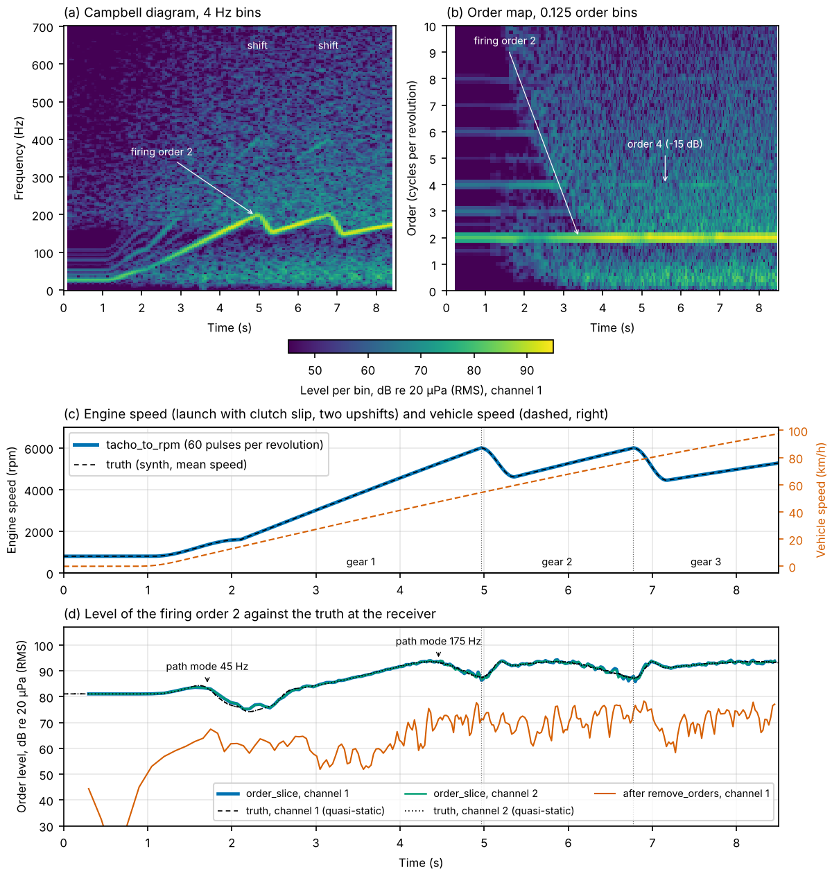
A synthetic four-cylinder engine run-up from rota_order.synth.synth_scenario("ice_runup"): launch from idle with clutch slip, two upshifts, combustion bursts, a modal transfer path, engine broadband, road noise and rumble, two receiver channels. Campbell diagram and order map, the speed from the tachometer against the truth, and the level of the firing order against the truth at the receiver, before and after remove_orders (examples/05_realistic_engine_audio.py).
Worked analysis
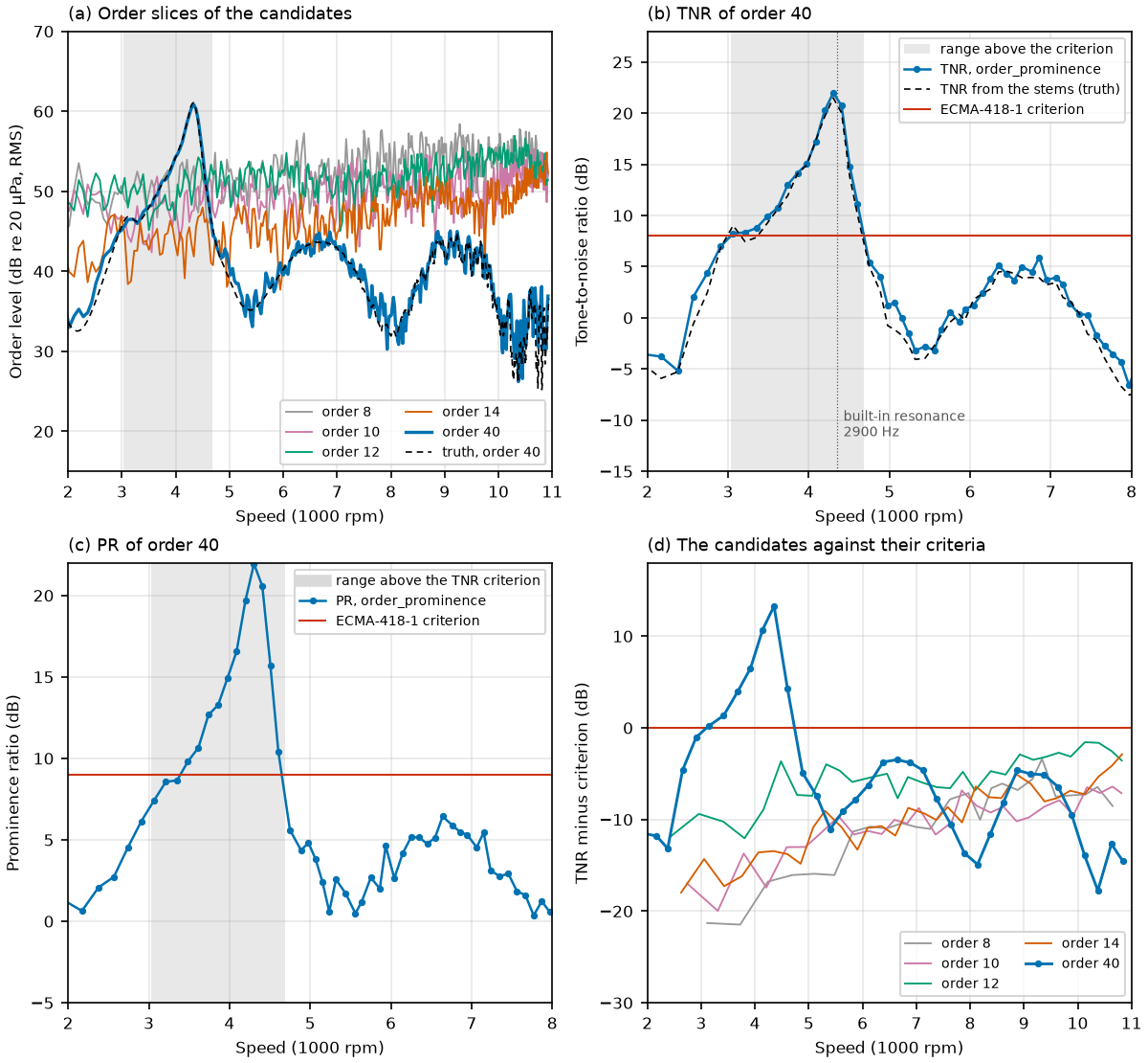
docs/worked_example.md follows one analysis from a run-up recording with a tonal complaint to a conclusion an engineer can act on: speed, overview (A-weighted level, 1/3-octave bands, order map), diagnosis of the prominent order with the ECMA-418-1 tone-to-noise and prominence ratios, extraction and a what-if reduction of that order, the effect on loudness, sharpness and ECMA-418-2 tonality computed with optional open-source toolboxes, and the result checked against the truth built into the synthetic signal, with audio before and after.
Plotting
rota_order.plot draws the standard figure of a result in one call, named like the function that computed it, and returns the Matplotlib Axes for anything else you want to change. Labels carry the unit, the dB reference and the amplitude convention; the reference is explicit (**rp.SOUND_PRESSURE for sound pressure in Pa):
import rota_order.plot as rp

m = ro.maps.rpm_order_map(x, fs, rpm, order_resolution=0.125, amplitude="rms")
ax = rp.rpm_order_map(m, **rp.SOUND_PRESSURE, mark_orders=(2, 4, 6))   # colour bar: dB re 20 µPa, RMS
ax.figure.savefig("order_map.png", dpi=150)                              # the rest is plain Matplotlib
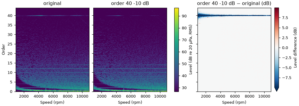
rp.order_slice({"before": s, "after": s_new}, relative_to="before")     # level change in dB
Here s and s_new are slices of the same order before and after a change (for example modify_orders and resynthesize). Matplotlib is an optional extra (pip install "rota-order[plot]"); import rota_order does not import it. docs/plotting.md shows one figure per function with the call that drew it (examples/11_plot_gallery.py).
Psychoacoustic toolboxes (optional)
rota_order.bridges calls MoSQITo, the Sottek hearing model or SQAT in one line, on rota-order's conventions (sound pressure in Pa, any sampling rate, calibration factor), and the vs_rpm method of the result bins it along rpm:
from rota_order import bridges

loud = bridges.mosqito.loudness(x, fs, calibration=cal)        # ISO 532-1:2017, sone
n5 = loud.vs_rpm(rpm, t_rpm, bin_width=250.0)                  # N5 per rpm bin, start-up skipped
ton = bridges.sottek_hearing_model.tonality(x, fs, calibration=cal).vs_rpm(rpm, t_rpm)   # ECMA-418-2:2025, tu_HMS
A bridge module is named exactly like the toolbox it wraps (mosqito, sottek_hearing_model, sqat), so the quantity and the toolbox are visible in the same line; a short alias is up to you (from rota_order.bridges import sottek_hearing_model as shm). rpm is the speed in rpm at the times t_rpm in s, on the time axis of x. vs_rpm applies the start-up exclusion and the aggregation recommended for the metric (any keyword of rota_order.slices.metric_vs_rpm overrides them), and the binned result carries the name, unit and source of the metric. For full control call rota_order.slices.metric_vs_rpm(m.values, m.t, rpm, t_rpm, ...) on the metric m yourself.
The toolboxes are never vendored or required; without one, the call raises ImportError with the install command. rota-order does not include, copy or redistribute any of their code: each keeps its own licence, and you install it yourself. Please cite the toolbox you use as its authors ask:
| Module | Toolbox | Licence | Needs | Cite |
|---|---|---|---|---|
rota_order.bridges.mosqito |
MoSQITo 1.2.1: ISO 532-1 loudness, DIN 45692 sharpness, Daniel & Weber roughness | Apache-2.0 | pip install mosqito (and matplotlib) |
Green Forge Coop (2024). MOSQITO, version 1.2.1. Zenodo. doi:10.5281/zenodo.11026796 |
rota_order.bridges.sottek_hearing_model |
sottek-hearing-model 0.1.14: ECMA-418-2:2025 tonality, loudness, roughness | AGPL-3.0-only | pip install sottek-hearing-model, Python 3.11 or later |
Lotinga, M. J. B., Torjussen, M., & Felix Greco, G. (2025). Verified implementations of the Sottek psychoacoustic Hearing Model standardised sound quality metrics (ECMA-418-2 loudness, tonality and roughness). Forum Acusticum / Euronoise 2025, Malaga. doi:10.61782/fa.2025.0951 |
rota_order.bridges.sqat |
SQAT v2.0 (MATLAB): ISO 532-1 loudness, DIN 45692 sharpness, Daniel & Weber roughness, ECMA-418-2:2025 tonality | GPL-3.0 (some files BSD-3-Clause or MIT) | a licensed MATLAB with the Signal Processing Toolbox, pip install matlabengine matching your MATLAB release, a SQAT checkout in ROTA_ORDER_SQAT_PATH |
Felix Greco, G., Merino-Martínez, R., Osses, A., & Lotinga, M. J. B. (2026). SQAT: a sound quality analysis toolbox for MATLAB. Zenodo. doi:10.5281/zenodo.7934709; Felix Greco, G., Merino-Martínez, R., Osses, A., & Langer, S. C. (2023). INTER-NOISE 2023. doi:10.3397/IN_2023_1075 |
The Sottek hearing model is AGPL-3.0-only: rota-order (GPL-3.0-or-later) may be used together with it, but whoever distributes the combination, or offers it to others over a network, must meet the AGPL-3.0 terms for the model's part. Examples 07, 08 and 10 use these bridges; example 09 runs SQAT in MATLAB in CI, and its README shows rota_order.bridges.sqat on a local MATLAB. Open-source implementations of psychoacoustic metrics, with the standard and edition each follows, are listed in LISQM.
Listen
The recordings below are synthetic (no measured data) and are written by examples/05_realistic_engine_audio.py and examples/06_electric_drive_audio.py: 16-bit WAV at 32 kHz, all with the same scaling (4 Pa is digital full scale), so levels can be compared between files.
- engine_runup.wav: the engine run-up as recorded (two channels).
- engine_runup_orders_removed.wav: the residual after
remove_orders: engine broadband, road noise, rumble and what is not periodic in the combustion bursts. - engine_runup_orders_only.wav: the extracted engine orders.
- engine_runup_faster.wav: the same recording with the apparent engine speed raised by 15 % (
remap_rpm, thenresynthesizewith the residual kept). - electric_runup.wav: an electric drive run-up: motor orders and gear whine, a dithered 10 kHz inverter carrier with sidebands, two fixed tones, road noise and rumble. The tonal lines are weak against the broadband.
- electric_runup_motor_orders_removed.wav: after removing the motor and gear orders; the inverter sidebands are not orders and remain.
- electric_runup_whine_only.wav: the extracted motor and gear orders.
Tacholess speed
rota_order.speed.rpm_from_ridge estimates the speed from the signal alone with a comb of orders and a dynamic-programming ridge. Give it the orders the machine shows: the comb, not the data, decides between a speed and its octaves. For a four-stroke engine with N cylinders the firing order N/2 and its harmonics dominate, so use orders=(2, 4, 6) for four cylinders (the default (1, 2, 3, 4) then reads twice the crankshaft speed), (1.5, 3, 4.5) for three and (3, 6, 9) for six. Set rpm_range from a priori knowledge (idle speed to redline). The window adapts to the sweep by default (window="auto": 0.4 s, shorter for fast run-ups), and several channels are combined by averaging their power spectra. Each result carries a per-frame confidence (near 1 on a clean correct track, near 0 in noise) and a quality summary (median confidence, fraction of frames at a search bound, fraction of jumping frames, octave scores); a RidgeQualityWarning is issued when the track as a whole is likely wrong.
Conventions
- Units. Time in s, sampling rate and frequency in Hz, rotational speed in rev/min (rpm), shaft angle in revolutions, order in cycles per revolution, vehicle speed in km/h.
- Arrays. Signals have shape
(n,)or(n, ch). Every operator acts on each channel independently and linearly, so amplitude and phase relations between channels are preserved. - Amplitude. Peak or RMS is always stated in the docstring and, where there is a choice, selected by an explicit
amplitudeargument ("peak"or"rms"). - No hidden constants. Gains, calibration factors and reference pressures are passed explicitly. They are never built into a function.
- Randomness. Every random process takes a
numpy.random.Generatoror an integer seed. - Estimators. Functions that estimate quantities (speed, order amplitude) are meant to return a confidence and to report when a search boundary was reached.
Design principles
- Independent implementation: algorithms follow public literature only (see Independence statement).
- Verifiable: each function is tested on synthetic signals with known analytic ground truth.
- Transparent: docstrings give the literature, the amplitude definition and the units.
- Plain Python: snake_case functions, NumPy arrays as input and output, computation separate from plotting.
- Interoperable: results can be passed on to open-source psychoacoustic tools; examples 07 to 09 link rota-order to MoSQITo, sottek-hearing-model and SQAT. rota-order does not depend on them. Open-source implementations of psychoacoustic metrics, with the standard and edition each follows, are listed in LISQM.
- Multichannel first: operators are linear per channel (see Conventions).
- Reproducible: seedable randomness, and planned JSON sidecar files recording the parameters of each resynthesis.
- No hidden constants.
Validation
Analytic ground truth from rota_order.synth is the first reference: every test signal comes with its true speed, shaft angle, and amplitude and phase of each order. A black-box comparison with MATLAB's documented public functions, all parameters explicit, is the second reference: it runs in CI (workflow matlab-reference, see validation/README.md) and compares physical quantities (speed curves, order amplitudes along a ridge, Vold-Kalman waveforms and bandwidth), not map cells; when the two disagree, the analytic truth decides. Its output stays in the workflow artifact and is not published in the repository until the licence terms are confirmed. Resynthesis is tested by round trip: synthesise, analyse, compare with the input table. Continuous integration runs pytest only.
The design document defines 14 validation signals (T1 to T14). Version 0.1 covers T1 (single order, constant amplitude, linear run-up), T2 (several orders, a fixed-frequency resonance, noise), T5 (multi-pulse tachometer with jitter and dropped pulses) and T14 (low-speed start from idle with orders half an order apart). Version 0.2 adds T3 (exponential run-down), T4 (crossing orders on two shafts), T6 (fast run-up), T8 (twin shafts 0.5–4 % apart), T10 (true speed outside the search range), T12 (order removal) and T13 (extraction error versus speed-reference error). Version 0.3 adds T9 (order table → synthesis → analysis → table round trip, tests/test_ordertable.py) and T11 (broadband synthesis: PSD accuracy and no frame-rate pumping, tests/test_broadband.py). Version 0.4 adds stress tests on realistic scenarios (validation/stress.md). Cases and measured results: validation/README.md.
Tolerances (the analytic column is enforced by the test suite; the black-box column is the target of the CI comparison):
| Quantity | Against analytic truth | Against black-box reference |
|---|---|---|
| Speed, median relative error | <= 0.1 % | <= 0.1 % |
| Tacholess speed, fraction of frames within 3 % (steady or slowly rising) | >= 90 % | within 5 percentage points |
| Order amplitude, stationary segments | <= 0.2 dB | <= 0.5 dB |
| Order amplitude near a resonance | <= 1 dB | <= 1 dB |
| Order waveform correlation (edges removed) | >= 0.99 | >= 0.99 |
| Vold-Kalman -3 dB bandwidth | within 5 % of the set value | within 5 % |
| Order-table round trip, amplitude (T9) | <= 0.2 dB | not compared |
| Remaining energy of a removed order in the residual (T12) | <= -20 dB | not compared |
| Frame-rate pumping of broadband synthesis (T11) | <= 1 dB | not compared |
All rows of the analytic column are met by the current release; measured values are in validation/README.md.
Independence statement
rota-order is an independent academic project. It is not affiliated with, endorsed by, or supported by MathWorks or any commercial software vendor. MATLAB is a registered trademark of The MathWorks, Inc.
All algorithms are implemented from the published literature cited in each docstring, and rota-order reads no proprietary file formats.
License
rota-order is free software: you can redistribute it and/or modify it under the terms of the GNU General Public License as published by the Free Software Foundation, either version 3 of the License, or (at your option) any later version. See LICENSE.
Citation
See CITATION.cff (GitHub shows it as "Cite this repository"). A Zenodo DOI is planned for v1.0.
Acknowledgements
rota-order is designed, implemented and maintained by Zhenxian Li. Claude (Anthropic) was used as an assistant during development.
1 maintainer

Metadata
1 maintainer
Release files for rota-order 0.8.0
For a detailed explanation of source distributions (sdists) and built distributions (wheels), please see the package formats documentation.
Source distribution (sdist)
| File | Size | Uploaded | Provenance | Actions |
|---|---|---|---|---|
| rota_order-0.8.0.tar.gz | 611.2 kB | With provenance | Details for rota_order-0.8.0.tar.gz |
Built distribution (wheel)
| File | Interpreter | ABI | Platform | Actions Reset |
|---|---|---|---|---|
| rota_order-0.8.0-py3-none-any.whl | Python 3 | none | any | Details for rota_order-0.8.0-py3-none-any.whl |
Total release size: 963.0 kB
Release files / rota_order-0.8.0.tar.gz
| Download URL | rota_order-0.8.0.tar.gz |
|---|---|
| Size | 611.2 kB |
| Tags | Source |
|
SHA-256 checksum How to use checksums |
4145a1ecf58430c1486c44fb5916244b5da7a0df4330584876c297f9a8c44701
|
|
BLAKE2b-256 checksum How to use checksums |
e0424d47af4160585f435bf6b6371cd74164680446ab3de072d71c35d8930b65
|
| Upload date | |
|
Uploaded using Trusted Publishing? What is trusted publishing? |
Yes |
| Uploaded via |
twine/7.0.0 CPython/3.13.16
|
Provenance
Provenance describes where a file came from. On PyPI, provenance is shared via attestations, which provide a verifiable record of the build or publishing details. View details, limitations and caveats.


PyPI Publish Attestation
PyPI verified that this artifact, at this checksum, originated from the publisher listed below.
Signed by GitHub Actions, verified by PyPI on Oct 28, 2026.
Transparency logRelease files / rota_order-0.8.0-py3-none-any.whl
| Download URL | rota_order-0.8.0-py3-none-any.whl |
|---|---|
| Size | 351.8 kB |
| Tags | Python 3 |
|
SHA-256 checksum How to use checksums |
9b3ed7c3c07099be6d4ab32950d46a236dc0213fba24ebc29a760e20517e03b3
|
|
BLAKE2b-256 checksum How to use checksums |
b9c82e3f8e429a735c59ec7e564698b41063256eb25e2cee4ea92352ad66c83c
|
| Upload date | |
|
Uploaded using Trusted Publishing? What is trusted publishing? |
Yes |
| Uploaded via |
twine/7.0.0 CPython/3.13.16
|
Provenance
Provenance describes where a file came from. On PyPI, provenance is shared via attestations, which provide a verifiable record of the build or publishing details. View details, limitations and caveats.
PyPI Publish Attestation
PyPI verified that this artifact, at this checksum, originated from the publisher listed below.
Signed by GitHub Actions, verified by PyPI on Oct 28, 2026.
Transparency logSecurity for rota-order 0.8.0
Provenance
Provenance describes where a file came from. On PyPI, provenance is shared via attestations, which provide a verifiable record of the build or publishing details. View details, limitations and caveats.
Full provenance
All 2 files in this release have been uploaded with provenance metadata.
Attestation for rota_order-0.8.0.tar.gz
PyPI Publish Attestation
PyPI verified that this artifact, at this checksum, originated from the publisher listed below.
Signed by GitHub Actions, verified by PyPI on Oct 28, 2026.
Transparency logA note on package security
PyPI is a repository for distributing packages, not a service for auditing them. While third-party security researchers and our staff do their best to detect and remove malicious packages, PyPI cannot guarantee the quality, security or suitability of any given package.
To learn more about protecting yourself from malicious actors, visit our package security documentation.














