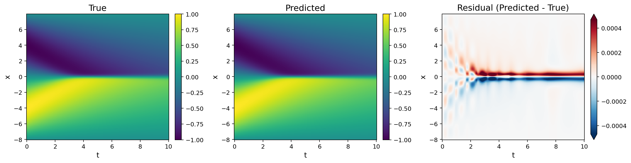





KD discovers the governing partial differential equation from a field
sampled on a spatiotemporal grid. The same Model.fit also takes a plain
feature table and returns a scalar expression y = f(X).
Five in-house algorithms (SGA, DLGA, DISCOVER, EqGPT, LLM4ED) and two external
baselines (PySR, PySINDy) run behind one kd.Model API, with a common dataset
interface, visualization and HTML reports.
Install
In an activated Python 3.11+ environment, install with uv:
uv pip install sail-kd --torch-backend=auto
The option selects the PyTorch build for your hardware. See
Installation
for environment setup, pip installation, CPU/CUDA builds and optional components.
For a source checkout, clone this repository's trunk branch and run uv sync.
Quick start
Discover Burgers' equation from the bundled 256 × 201 field:
import kd

dataset = kd.load_burgers()
model = kd.Model(algorithm="sga", generations=5, seed=0)
model.fit(dataset)

print(model.result_.equation)  # u_t = -u*u_x + 0.1002*u_xx
The five-generation search recovers
$$u_t = -u,u_x + 0.1002,u_{xx}$$
against the benchmark equation $u_t = -u,u_x + 0.1,u_{xx}$.
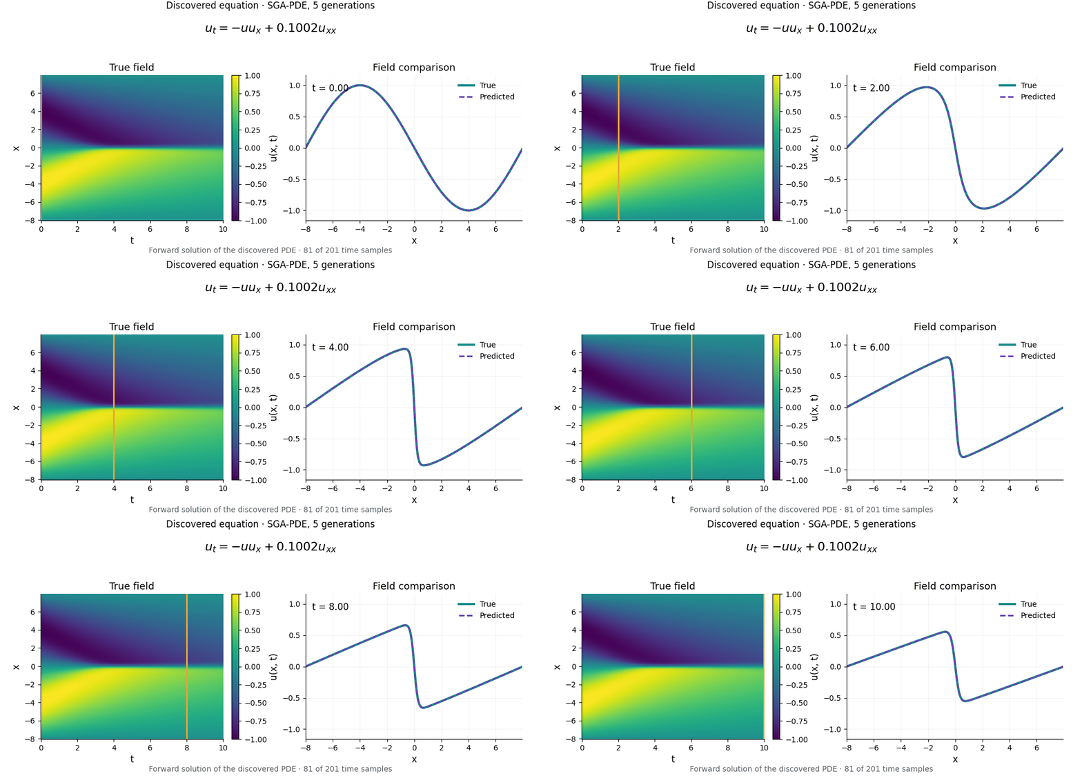
The animation follows the field through time. The marker on the left selects the profile shown on the right, where the observations are compared with the forward solution of the discovered PDE. The solution uses this fit's coefficients, starts from the dataset's initial condition and uses its periodic spatial boundary. The full field comparison includes the residual.
First fit
explains the result and its diagnostics. model.report("out/burgers") writes an
HTML report with convergence, residuals, field comparisons and search diagnostics.
Your own data enters through kd.load, which takes a catalog id or a file path.
Inspect a file's arrays first, then name its coordinates and fields:
kd.inspect_file("run.mat")
dataset = kd.load("run.mat", coords={"x": "x", "t": "t"},
                  fields={"u": "usol"}, lhs="u_t")
Use your own data
also covers registered layouts such as PDEBench HDF5, sample selection and
PDEDataset.from_arrays for arrays already in memory.
Algorithms
The five in-house algorithms are refactored re-implementations of methods
developed in the Scientific Artificial Intelligence Lab. Swap the algorithm=
string to switch; all seven share one dataset interface and one result object.
Each linked page covers the method, its parameters and setup.
| Algorithm | algorithm= |
Origin | Approach |
|---|---|---|---|
| SGA-PDE | "sga" |
Chen et al. 2022 | Genetic algorithm over symbolic expression trees |
| DLGA-PDE | "dlga" |
Xu et al. 2020 | Neural-network surrogate + genetic algorithm |
| DISCOVER | "discover" |
Du et al. 2024 | LSTM controller + policy gradient |
| EqGPT | "eqgpt" |
Xu et al. 2025 | Pretrained GPT proposes candidate PDEs, followed by reward-guided fine-tuning |
| LLM4ED | "llm4ed" |
Du et al. 2024 | An LLM proposes candidate equations as text, scored by a sparse-regression reward |
| PySR | "pysr" |
External, Cranmer 2023 | Genetic programming over expression trees |
| PySINDy | "pysindy" |
External, de Silva et al. 2020 | Native STLSQ sparse regression over a KD term library |
DISCOVER and PySR also accept feature tables. SGA-PDE and PySINDy support
sketches that specify known terms and constrain
the unknown remainder. Algorithm settings can be passed as Model keywords;
the API reference
documents their types, defaults and programmatic configuration schemas.
Tabular data
Model.fit also accepts a TabularDataset: a plain feature table, searched for
y = f(X) with no fields, no derivatives and no term library to supply. The
example below uses the bundled TLC-CC measurements, 74 chromatography conditions.
import kd

dataset = kd.load_tlc_cc(target="start")  # X = (R_F, r), y = V_S
model = kd.Model("discover", generations=100, seed=0,
                 batch_size=500, reward_alpha=0.005, max_length=15).fit(dataset)

for entry in model.result_.pareto_front():
    print(entry.complexity, entry.loss, entry.scale, entry.expression)
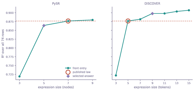
The Pareto front records accuracy and expression size. Each entry holds the raw
candidate in entry.expression and its fitted outer coefficient in entry.scale;
both are needed to read the fitted expression. DISCOVER and PySR run in tabular
mode. Column chromatography
compares their fronts and the recovered coefficients with the published formula.
Examples and datasets
 Breaking waves
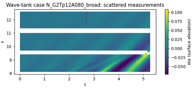
Reproduce the published EqGPT equation on 12 wave-tank experiments. |
 Column chromatography
Compare DISCOVER and PySR on 74 measured conditions and locate the published formula on each Pareto front. |
For a longer PDE search, the KdV walkthrough follows 200 generations of SGA-PDE and explains the discovered terms and report.
The simulated datasets come from this lab's PDE-discovery papers, including SGA-PDE, EqGPT and LLM4ED. The catalog runs from Burgers and KdV to 2D Burgers, Klein-Gordon and the Fisher family. KD also bundles two experimental datasets: wave-tank surface elevations and chromatography retention volumes, used with the permission of the authors. The dataset catalog provides equations, grids, measurement protocols, sources and licenses; the dataset API also covers synthetic generators and downloads.
All tutorials and runnable scripts cover every algorithm, including tabular regression and algorithm comparison.
Discovery with a sketch
When part of the law is already known, fit(dataset, sketch=...) states that
part and searches the remainder. A pinned term is subtracted from the regression
target before the search and restored with its coefficient in the solution.
An anchored term fixes the structure while leaving its coefficient free.
A hole declares how many terms may fill it and what forms they may take,
including derivative order, operators, fields and axes.
SGA-PDE and PySINDy accept sketches. The Burgers sketch example pins the advection term, searches for the missing diffusion term and explains how the result is checked against the sketch and the data.
Further use
| Capability | Guide or example |
|---|---|
Experimental controller: configure a language-model endpoint, search a dataset and receive a Markdown report with kd-agent |
Controller guide |
| Figures and HTML reports: inspect convergence, residuals, field comparisons and algorithm-specific diagnostics | Visualization |
| Checkpoint and resume: save search state and continue from a recorded checkpoint | Resume guide |
| Batch experiments: run an algorithm × dataset plan with recorded environments and consensus reports | Batch guide |
| Term evaluation: fit candidate terms or validate them with per-term rejection reports | Term API |
| Dataset preview: inspect axes, spacing, field statistics and the left-hand side before searching | Data requirements |
Citation and acknowledgements
For research using KD, cite the original works for the methods and datasets you use. The five lab algorithms are refactored re-implementations of these methods; their algorithm pages provide the papers and references:
- SGA-PDE: Chen et al., Phys. Rev. Research 4, 023174 (2022); original code.
- DLGA-PDE: Xu et al. (2020); paper and references.
- DISCOVER: Du et al. (2024); original code.
- EqGPT: Xu et al., Nat Commun 16, 10255 (2025); original code.
- LLM4ED: Du et al., Phys. Fluids 36, 097121 (2024); original code.
KD also builds on PySR, PySINDy, SymPy and PyTorch. Dataset attribution and redistribution terms are in NOTICE.
License
Apache-2.0. Copyright 2026 Mao, Hao and the Scientific Artificial Intelligence Lab.
1 maintainer

Metadata
1 maintainer
Release files for sail-kd 0.8.1
For a detailed explanation of source distributions (sdists) and built distributions (wheels), please see the package formats documentation.
Source distribution (sdist)
| File | Size | Uploaded | |
|---|---|---|---|
| sail_kd-0.8.1.tar.gz | 20.2 MB | Details |
Built distribution (wheel)
| File | Interpreter | ABI | Platform | Reset |
|---|---|---|---|---|
| sail_kd-0.8.1-py3-none-any.whl | Python 3 | none | any | Details |
Total release size: 40.5 MB
Release files / sail_kd-0.8.1.tar.gz
| Download URL | sail_kd-0.8.1.tar.gz |
|---|---|
| Size | 20.2 MB |
| Tags | Source |
|
SHA-256 checksum How to use checksums |
74be65a3e80d8bd96f3b273004203b4fc20461da4b71e5e26f107854ad3f0bf3
|
|
BLAKE2b-256 checksum How to use checksums |
54030b3c8700b4845905e3099b1bf44ccb3354aec3ccfe821b68f5483ed068c7
|
| Upload date | |
|
Uploaded using Trusted Publishing? What is trusted publishing? |
No |
| Uploaded via |
uv/0.11.8 {"installer":{"name":"uv","version":"0.11.8","subcommand":["publish"]},"python":null,"implementation":{"name":null,"version":null},"distro":{"name":"Ubuntu","version":"24.04","id":"noble","libc":null},"system":{"name":null,"release":null},"cpu":null,"openssl_version":null,"setuptools_version":null,"rustc_version":null,"ci":null}
|
Release files / sail_kd-0.8.1-py3-none-any.whl
| Download URL | sail_kd-0.8.1-py3-none-any.whl |
|---|---|
| Size | 20.3 MB |
| Tags | Python 3 |
|
SHA-256 checksum How to use checksums |
a5e3585201696f54323a4f0b936d75e4226b06dabdb65f3130028bf4a642d859
|
|
BLAKE2b-256 checksum How to use checksums |
72e6317c97a6f7484c9ceb950917695f3820782e77f8aa330ce6d8245f845225
|
| Upload date | |
|
Uploaded using Trusted Publishing? What is trusted publishing? |
No |
| Uploaded via |
uv/0.11.8 {"installer":{"name":"uv","version":"0.11.8","subcommand":["publish"]},"python":null,"implementation":{"name":null,"version":null},"distro":{"name":"Ubuntu","version":"24.04","id":"noble","libc":null},"system":{"name":null,"release":null},"cpu":null,"openssl_version":null,"setuptools_version":null,"rustc_version":null,"ci":null}
|