
scikit-complexity
| Category | Tools |
|---|---|
| Development |     |
| Testing |    |
| Security |   |
| Automation |   |
| Package |    |
| Documentation |  |
| Communication |  |
Overview
scikit-complexity lets you describe a model from any science in a few lines, and takes care of the rest: it works
out the mathematics, picks a solver, runs the simulation, and streams it live to the Rerun viewer.
Flocks, epidemics, markets, fluids, neural networks and cellular automata are usually written in separate tools with separate conventions. Here they share one small vocabulary, in the spirit of scikit-learn: elements carry state, interactions change it through laws, and systems nest and compose. Learn it once, and every field opens up.
 Physics Decaying 2D turbulence |
 Chemistry Gray-Scott patterns |
 Biology Boids flocking |
 Economics Sugarscape |
 Engineering Nagel-Schreckenberg traffic |
 Mathematics Julia sets |
 Computer science Game of Life |
 Social science Schelling segregation |
A few of the 549 ready-to-run models, each with a documented example in the gallery.
Features
- Every kind of dynamics, one interface. Differential equations, stochastic processes, jump processes, discrete maps, cellular automata, agents, networks and hypergraphs, fields and PDEs, quantum systems, and models that learn by gradient descent.
- The form of your model is inferred. Write the laws; the framework decides whether it is an ODE, an SDE or a jump process, and compiles it for NumPy, Numba, or JAX.
- Symbols when you want them, code when you don't. Laws are Sage symbolic expressions you can inspect and solve exactly, or plain Python functions.
- Watch it run. Stream any simulation to Rerun in real time, and change its parameters while it runs.
- Analysis included. Nearly 50 analyses, from Lyapunov exponents and entropy to network motifs, scaling laws and system identification, plus experiments for parameter sweeps, sensitivity, calibration and basin stability.
- Standing on mature libraries. SciPy, NetworkX, Mesa, LAMMPS, QuTiP, JAX and others do the heavy lifting.
- Extend it, don't fork it. Models are written with the same public classes you use, so each one doubles as an example for your own.
Installation
scikit-complexity supports Python 3.12, 3.13, and 3.14 on Linux and on macOS 13 or later with Apple silicon, and is
available on PyPI. On Python 3.14 the install builds memory-allocator from source, so it needs a C compiler:
pip install scikit-complexity
The installation includes Sage through the passagemath distributions, LAMMPS, Mesa, Numba, JAX, and Rerun. Windows has no passagemath wheels, so on Windows the package runs in WSL.
For development, clone the repository and install the project with PDM:
git clone https://github.com/georgedouzas/scikit-complexity.git
cd scikit-complexity
pdm install
Usage
There are two ways to use the library. Select a prebuilt model from the catalog by its name, or build a custom model
from the general classes of skcomplex.core.
Select a prebuilt model
Every one of the more than 500 prebuilt models has a description, tags, parameters, and references, so you can browse the catalog from Python:
from skcomplex.models import catalog, describe

for model in catalog(field='biology/ecology'):
    print(model.name, '-', model.description)

print([model.name for model in catalog() if 'oscillation' in model.tags])

entry = describe('lotka_volterra')
print(entry.description, entry.formalism, entry.parameters, entry.references)
Run any of them in one line:
from skcomplex.models import run

trajectory = run('sir').trajectory_
print(trajectory.values('I.n').max().round())
create returns the system of a model with the arguments you choose, so you can simulate it with settings of your own:
from skcomplex.engine.runtime import Simulation
from skcomplex.models import create

system = create('lotka_volterra', r=1.5)
trajectory = Simulation(system, dt=0.1).check().prepare().run(until=50).trajectory_
print(round(float(trajectory.values('prey.n').max())))
Each run can stream to the Rerun viewer:
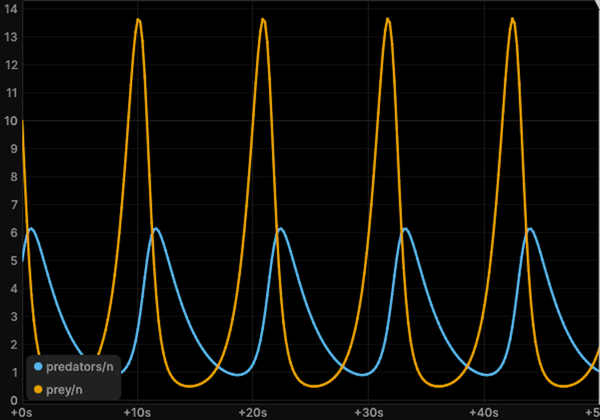 lotka_volterraPrey and predators cycle |
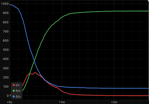 sirAn epidemic rises and fades |
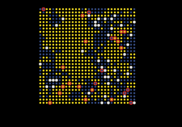 wolf_sheepWolves, sheep and grass on a grid |
The catalog lists every model by field and tag, and the page of each model shows the classes it is built from.
Build a custom model
A custom model needs only the core. An element declares its states, and an interaction declares its roles and returns
its laws, where the namespace s holds the symbols of its parameters and of the elements bound to its roles. A predator
and prey model takes one element class, the general RateInteraction, and one new interaction:
from typing import Annotated

from skcomplex.core.elements import Element
from skcomplex.core.interactions import Interaction, RateInteraction
from skcomplex.core.laws import RateLaw
from skcomplex.core.system import System
from skcomplex.engine.runtime import Simulation
from skcomplex.specs import ParameterSpec, RoleSpec, StateSpec


class PopulationElement(Element):
    def __init__(self, label, visual=None, *, n: Annotated[float, StateSpec()] = 1.0):
        super().__init__(label, visual=visual)
        self.n = n


class PredationInteraction(Interaction):
    def __init__(
        self,
        label,
        *,
        predator: Annotated[str, RoleSpec(states=('n',))],
        prey: Annotated[str, RoleSpec(states=('n',))],
        a: Annotated[float, ParameterSpec()] = 0.4,
        b: Annotated[float, ParameterSpec()] = 0.1,
    ):
        super().__init__(label)
        self.predator = predator
        self.prey = prey
        self.a = a
        self.b = b

    def _get_laws(self, s):
        contacts = s.predator.n * s.prey.n
        return [RateLaw(s.prey.n, -s.a * contacts), RateLaw(s.predator.n, s.b * contacts)]


system = System(
    elements=[PopulationElement('rabbits', n=40), PopulationElement('foxes', n=9)],
    interactions=[
        RateInteraction('growth', target='rabbits', state='n', rate=lambda s: 1.1 * s.target.n * (1 - s.target.n / 1000)),
        PredationInteraction('hunt', predator='foxes', prey='rabbits'),
        RateInteraction('death', target='foxes', state='n', rate=lambda s: -0.4 * s.target.n),
    ],
)
trajectory = Simulation(system, dt=0.05).check().prepare().run(until=30).trajectory_
print(round(float(trajectory.values('rabbits.n').max())))
A RerunObserver records the run for the Rerun viewer, and RerunObserver('predators', spawn=True) opens the viewer
during the run. A RealTimeClock paces the run against wall time:
import tempfile
from pathlib import Path

from skcomplex.engine.runtime import RealTimeClock
from skcomplex.engine.viz import RerunObserver

recording = Path(tempfile.mkdtemp()) / 'predators.rrd'
simulation = Simulation(
    system,
    dt=0.05,
    clock=RealTimeClock(speed=20.0),
    observers=[RerunObserver('predators', save_path=recording)],
).check().prepare()
print(simulation.run(until=30).trajectory_.times[-1])
A simulation started with start runs in the background, and its parameters can change while it runs:
simulation = Simulation(system, dt=0.05, clock=RealTimeClock(speed=20.0)).check().prepare().start(until=30)
simulation.update_parameters({'hunt.a': 0.2})
simulation.wait()
Adding a process takes one more interaction, and SymbolicAnalysis shows the equations of the system:
from sage.all__sagemath_symbolics import oo
from sage.sets.real_set import RealSet

from skcomplex.analysis import SymbolicAnalysis


class HarvestInteraction(Interaction):
    def __init__(
        self,
        label,
        *,
        target: Annotated[str, RoleSpec(states=('n',))],
        h: Annotated[float, ParameterSpec(domain=RealSet.closed_open(0, oo))] = 0.1,
    ):
        super().__init__(label)
        self.target = target
        self.h = h

    def _get_laws(self, s):
        return [RateLaw(s.target.n, -s.h * s.target.n)]


harvested = System(
    elements=[PopulationElement('fish', n=500)],
    interactions=[
        RateInteraction('growth', target='fish', state='n', rate=lambda s: 0.5 * s.target.n * (1 - s.target.n / 1000)),
        HarvestInteraction('fishing', target='fish', h=0.1),
    ],
)
print(SymbolicAnalysis().check().prepare(harvested).run().equations_['fish.n'])
Find out which components fit
An interaction states what it needs from each role, and an element states what it carries. Ask them before you build:
hunt = PredationInteraction('hunt', predator='foxes', prey='rabbits')
print(hunt.get_requirements().roles['prey'].states, list(PopulationElement('rabbits').get_states()))
When a role is bound to an element without the state it reads, validation names the role, the state, and the fix:
from skcomplex.engine.compile import PassCompiler


class TankElement(Element):
    def __init__(self, label, visual=None, *, level: Annotated[float, StateSpec()] = 1.0):
        super().__init__(label, visual=visual)
        self.level = level


wrong = System(
    elements=[TankElement('tank'), PopulationElement('foxes')],
    interactions=[PredationInteraction('hunt', predator='foxes', prey='tank')],
)
print(PassCompiler().check().prepare(wrong).report_.issues[0].text)
The compatibility page lists every element, interaction, law, solver, and backend, and the user guide walks through the choices in order.
Spec-driven development
The project's engineering constitution lives in openspec/constitution.md and binds all work. The
project uses OpenSpec for spec-driven development, and
openspec/config.yaml names the constitution as binding.
1 maintainer

Metadata
1 maintainer
Release files for scikit-complexity 0.4.0
For a detailed explanation of source distributions (sdists) and built distributions (wheels), please see the package formats documentation.
Source distribution (sdist)
| File | Size | Uploaded | Provenance | Actions |
|---|---|---|---|---|
| scikit_complexity-0.4.0.tar.gz | 3.1 MB | With provenance | Details for scikit_complexity-0.4.0.tar.gz |
Built distribution (wheel)
| File | Interpreter | ABI | Platform | Actions Reset |
|---|---|---|---|---|
| scikit_complexity-0.4.0-py3-none-any.whl | Python 3 | none | any | Details for scikit_complexity-0.4.0-py3-none-any.whl |
Total release size: 6.5 MB
Release files / scikit_complexity-0.4.0.tar.gz
| Download URL | scikit_complexity-0.4.0.tar.gz |
|---|---|
| Size | 3.1 MB |
| Tags | Source |
|
SHA-256 checksum How to use checksums |
98b830ce5a0882f6f864afe84e36ec4934d2ebc3939e084f0d9e23f49f96ac00
|
|
BLAKE2b-256 checksum How to use checksums |
6eb61c939c54f27dfefa6a589bf9a28c31e36390ca33f6a3d83fdebdcfac296d
|
| Upload date | |
|
Uploaded using Trusted Publishing? What is trusted publishing? |
Yes |
| Uploaded via |
twine/7.0.0 CPython/3.13.16
|
Provenance
Provenance describes where a file came from. On PyPI, provenance is shared via attestations, which provide a verifiable record of the build or publishing details. View details, limitations and caveats.


PyPI Publish Attestation
PyPI verified that this artifact, at this checksum, originated from the publisher listed below.
Signed by GitHub Actions, verified by PyPI on Nov 5, 2026.
Transparency logRelease files / scikit_complexity-0.4.0-py3-none-any.whl
| Download URL | scikit_complexity-0.4.0-py3-none-any.whl |
|---|---|
| Size | 3.4 MB |
| Tags | Python 3 |
|
SHA-256 checksum How to use checksums |
ebc12188aac39133d09ab9139300e75b966fa3e62965e5248cafb30a8a509287
|
|
BLAKE2b-256 checksum How to use checksums |
c264426b387027542da5b7d946ec758ff77bb533c9ecc233c7f43d85d8cc4da2
|
| Upload date | |
|
Uploaded using Trusted Publishing? What is trusted publishing? |
Yes |
| Uploaded via |
twine/7.0.0 CPython/3.13.16
|
Provenance
Provenance describes where a file came from. On PyPI, provenance is shared via attestations, which provide a verifiable record of the build or publishing details. View details, limitations and caveats.
PyPI Publish Attestation
PyPI verified that this artifact, at this checksum, originated from the publisher listed below.
Signed by GitHub Actions, verified by PyPI on Nov 5, 2026.
Transparency logSecurity for scikit-complexity 0.4.0
Provenance
Provenance describes where a file came from. On PyPI, provenance is shared via attestations, which provide a verifiable record of the build or publishing details. View details, limitations and caveats.
Full provenance
Both files in this release have been uploaded with provenance metadata.
Attestation for scikit_complexity-0.4.0.tar.gz
PyPI Publish Attestation
PyPI verified that this artifact, at this checksum, originated from the publisher listed below.
Signed by GitHub Actions, verified by PyPI on Nov 5, 2026.
Transparency logA note on package security
PyPI is a repository for distributing packages, not a service for auditing them. While third-party security researchers and our staff do their best to detect and remove malicious packages, PyPI cannot guarantee the quality, security or suitability of any given package.
To learn more about protecting yourself from malicious actors, visit our package security documentation.














