
scope-profiler
This module provides a unified profiling system for Python applications, with optional integration of LIKWID markers using the pylikwid marker API for hardware performance counters.
It allows you to:
- Configure profiling globally via a singleton ProfilingConfig.
- Collect timing data via context-managed profiling regions.
- Use a clean decorator syntax to profile functions.
- Optionally record time traces in HDF5 files.
- Automatically initialize and close LIKWID markers only when needed, and store the resulting hardware counters and derived metrics in the same HDF5 file.
- Print aggregated summaries of all profiling regions.
Install
Install from PyPI:
pip install scope-profiler
Usage
To set up the configuration, create an instance of ProfilingConfig and add it to the ProfileManager, this should be done once at application startup and will persist until the program exits or is explicitly finalized (see below). Note that the config applies to any profiling contexts created (even in other files) after it has been initialized.
from scope_profiler import ProfileManager

# Setup global profiling configuration
ProfileManager.setup(
    use_likwid=False,
    recursive_profile=False,
)

# Profile the main() function with a decorator
@ProfileManager.profile("main")
def main():
    x = 0
    for i in range(10):
        # Profile each iteration with a context manager
        with ProfileManager.profile_region(region_name="iteration"):
            x += 1

# Call main
main()

# Finalize profiler
ProfileManager.finalize()
Execution:
❯ python test.py
profiling_data.h5  (1 rank(s))
  region     ranks  calls    total [s]      avg [s]      min [s]      max [s]      std [s]
  ----------------------------------------------------------------------------------------
  main           1      1   0.00150371   0.00150371   0.00150371   0.00150371            0
  iteration      1     10    3.832e-06    3.832e-07     2.08e-07     8.75e-07  2.24319e-07
  ----------------------------------------------------------------------------------------
  TOTAL                11   0.00150754

  Regions may nest, so the summed total can exceed the wall-clock time.
finalize() prints the same table as scope-profiler inspect and
ProfilingResults.print_summary(). Pass verbose=False to suppress it.
Inspecting a profiling file
scope-profiler inspect prints what is inside an HDF5 profiling file: the
full run metadata (host, CPU, loaded modules, Slurm job, environment) and one
statistics line per region, with no plotting dependencies needed.
scope-profiler inspect profiling_data.h5
==============================================================================
profiling_data.h5
2 rank(s), 4 region(s), 0.18 MiB, 0.0951538 s wall clock
==============================================================================

Metadata
  Run
    timestamp              : 2026-07-26T18:57:49
    user                   : mlindqvi
    hostname               : lrdn1234
  System
    chip_information       : AMD EPYC 9654 96-Core Processor
  Parallelism
    mpi_size               : 2
    omp_num_threads        : 8
    total_cores            : 16
  Slurm
    SLURM_JOB_ID           : 9988776
  Modules (4)
    profile/base
    gcc/12.3.0
    openmpi/4.1.6--gcc--12.3.0
    python/3.11.7

Regions (4)
  region    ranks  calls  total [s]    avg [s]     min [s]    max [s]      std [s]
  --------------------------------------------------------------------------------
  timestep      2      8   0.139235  0.0174044   0.0165256  0.0176325  0.000338551
  solve         2      8  0.0991292  0.0123911   0.0115046  0.0125382  0.000335212
  setup         2      2  0.0473326  0.0236663   0.0222938  0.0250388   0.00137254
  assemble      2      8  0.0399496  0.0049937  0.00484729  0.0050345   5.5882e-05
  --------------------------------------------------------------------------------
  TOTAL               26   0.325647
Long values such as PATH are clipped unless --full is passed, regions can
be filtered with --include/--exclude/--ranks, reordered with --sort,
and either section shown alone with --metadata-only / --regions-only.
The metadata can also be exported to JSON, with one entry per inspected file and no clipping:
scope-profiler inspect profiling_data.h5 --export-metadata metadata.json --quiet
from scope_profiler.inspection import write_metadata_json

write_metadata_json("profiling_data.h5", "metadata.json")
Example plots
scope-profiler pproc turns an HDF5 profiling file into Gantt, flame,
duration, and speedup charts (see Flame graphs below for
details). The plots here come from examples/generate_readme_figures.py, a
small mock timestep loop with nested and self-recursive regions, and are
saved to figures/:
python examples/generate_readme_figures.py
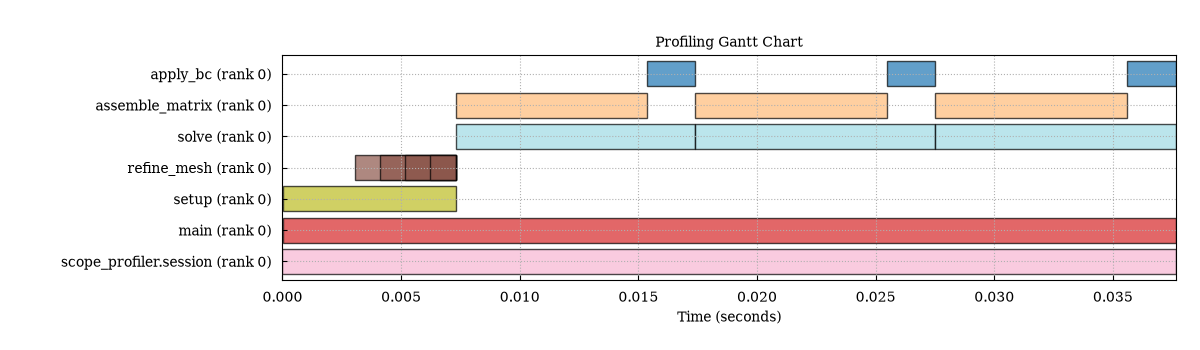
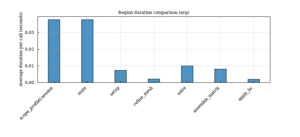
The flame graph for the same run is shown in Flame graphs below.
Overhead
The profiling overhead per call depends on the region type.
The benchmark below (examples/benchmark_overhead.py) measures each mode
against a bare function call:
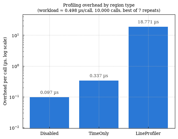
The default TimeOnly mode — nanosecond timestamps for every call — adds roughly 0.75 µs per instrumented call.
Profiling can also be fully deactivated at setup time
(deactivate_profiling=True) to reduce the overhead to ~0.03 µs — barely
above a bare function call — making it safe to leave instrumentation in
production code and toggle it on only when needed.
The LineProfiler mode is intentionally heavier (~41 µs/call) because
line_profiler traces every source line. It is designed for targeted
debugging of individual functions, not for always-on use in hot loops.
Recursive profiling of nested calls
You can profile nested Python calls from one decorated entrypoint:
from scope_profiler import ProfileManager

ProfileManager.setup(recursive_profile=True)


def leaf(x):
    return x + 1


def inner(x):
    return leaf(x) * 2


@ProfileManager.profile("entry")
def entry():
    return sum(inner(i) for i in range(3))


entry()
ProfileManager.finalize()
When enabled, the profiler records regions for nested calls using fully
qualified names (for example, my_module.inner), in addition to the main
decorated region.
Zero-instrumentation CLI profiling
You can profile a whole script without touching its source, similar to
python -m cProfile:
scope-profiler run my_script.py [script args...]
# equivalently: python -m scope_profiler run my_script.py [script args...]
Every Python function call the script makes is recorded as its own region
under a name derived from its module and qualified name, using the same
recursive tracer as recursive_profile=True above. By default only the
script's own code is instrumented (the standard library and installed
packages are skipped) to keep overhead low; pass --all to trace
everything. Results are written to profiling_data.h5 by default
(-o/--outfile to change it), and a per-region summary is printed unless
-q/--quiet is given.
See examples/ex_cli_profiling.py for a script with no scope-profiler
imports at all, run with:
scope-profiler run examples/ex_cli_profiling.py
Profiling self-recursive functions
A single region can also be safely re-entered by a recursive function - each call gets its own slot in the region's buffer, so nested calls don't overwrite each other's timing data. This works with both the decorator and context-manager forms:
from scope_profiler import ProfileManager

ProfileManager.setup()


@ProfileManager.profile("fibonacci")
def fibonacci(n):
    if n < 2:
        return n
    return fibonacci(n - 1) + fibonacci(n - 2)


def fibonacci_context_manager(n):
    with ProfileManager.profile_region("fibonacci_ctx"):
        if n < 2:
            return n
        return fibonacci_context_manager(n - 1) + fibonacci_context_manager(n - 2)


fibonacci(10)
fibonacci_context_manager(10)
ProfileManager.finalize()
Both fibonacci and fibonacci_ctx will report one call per recursive
invocation, each with correct, non-overlapping timing data.
Analysing results in Python
read_h5() loads a merged profiling file into a ProfilingResults, which
behaves like an ordered mapping of region name to region. Every duration and
timestamp it reports is in seconds:
from scope_profiler import read_h5

results = read_h5("profiling_data.h5")
results.print_summary()

# region       calls     total [s]       avg [s]       min [s]       max [s]
# ---------------------------------------------------------------------------
# setup            1       0.02401       0.02401       0.02401       0.02401
# timestep         5      0.062835      0.012567     0.0087755     0.0187844

solve = results["solve"]          # an MPIRegion: the region across all ranks
solve.num_calls                   # summed over ranks
solve.total_duration              # seconds
solve.average_durations()         # {rank: seconds}, for load imbalance
solve[0].durations                # every call on rank 0, as a numpy array
summary() returns the same table as a list of dicts, and to_dataframe()
returns it as a pandas DataFrame (one row per region, or per region and rank
with per_rank=True):
frame = results.to_dataframe().sort_values("total_duration", ascending=False)
per_rank = results.to_dataframe(per_rank=True)
include / exclude regexes select regions in get_regions(), summary(),
to_dataframe() and every plot_* function.
Building your own plots
For custom analysis, work from the individual calls instead of the
aggregates. events() returns one entry per recorded call, and
to_events_dataframe() returns the same as a pandas DataFrame. Timestamps
start at zero (the first region entry in the file), so they plot directly:
events = results.to_events_dataframe()
# columns: name, rank, call_index, start, end, duration   (seconds)

events.query("name == 'solve'")["duration"].hist(bins=50)
events.pivot_table(index="rank", columns="name", values="duration", aggfunc="sum")
Timestamps are measured from the start of the run, which setup() records.
results.run_start_time is that instant, and results.startup_time the gap to
the first profiled region — time the instrumentation never saw:
print(f"{results.startup_time:.3f} s before the first region was entered")
Files written without a start time (anything from before this existed) still
read fine: run_start_time is then None, startup_time is 0.0, and the
relative timeline falls back to the first region entry as before.
results.minimum_start_time, results.maximum_end_time and results.time_span
bound the profiled window, and results.call_stack(rank=0) hands back the
nesting the flame graph draws — one dict per call with depth and parent —
so you can render your own nested view:
for call in results.call_stack(rank=0):
    print(f"{'  ' * call['depth']}{call['name']}: {call['duration']:.6f} s")
To post-process in the same script that recorded the data, use
ProfileManager.read_results() after finalize() — it opens the file the
current configuration wrote (on rank 0 under MPI).
The tutorial notebooks cover this in depth: getting started, post-processing, visualization, profiling modes, custom analysis and building your own plots.
Flame graphs
Because each call - including recursive re-entries of the same region -
now has its own correctly nested (start, end) interval, the call stack can
be reconstructed straight from the timing data and rendered as a flame
graph, with recursion showing up as a narrowing tower of frames - as with
refine_mesh below, from the same run shown in Example plots:
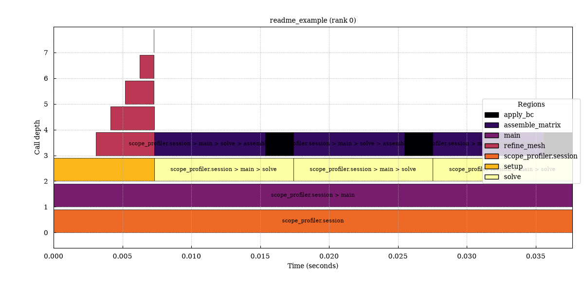
scope-profiler pproc generates flame_plot.png alongside the Gantt chart
for every run:
scope-profiler pproc profiling_data.h5 --show -o figures
Or programmatically:
from scope_profiler import read_h5, plot_flame

results = read_h5("profiling_data.h5")
plot_flame(results, filepath="flame_plot.png")
Gantt and flame charts (and plot_speedup) always color the same region the
same way. Pass --cmap (or cmap= on the plot_* functions) to use a
different matplotlib colormap
than the default tab20:
scope-profiler pproc profiling_data.h5 --cmap viridis -o figures
By default the flame graph covers rank 0, since it represents a single
execution's call stack; pass ranks=[...] to render one flame graph per
requested rank.
Exporting plot data
Every plot_* function accepts a data_filepath argument that writes the
exact data behind the chart to a file, so it can be re-parsed and re-plotted
later without the original HDF5 file. data_format selects "csv" (default)
or "json":
plot_gantt(results, filepath="gantt_plot.png", data_filepath="gantt_data.csv")
plot_gantt(
    results,
    filepath="gantt_plot.png",
    data_filepath="gantt_data.json",
    data_format="json",
)
The JSON payload additionally includes a colors map (region or file label
to #rrggbb) matching the colors used in the matplotlib plot, so a
JavaScript charting library like Plotly can reproduce the same look.
scope-profiler pproc --export-data does the same for every plot in one
run, writing gantt_data, flame_data, durations_data, and (for multiple
input files) speedup_data alongside the PNGs. Pass --export-data-format json to get .json files instead of the default .csv:
scope-profiler pproc profiling_data.h5 -o figures --export-data
scope-profiler pproc profiling_data.h5 -o figures --export-data --export-data-format json
Pass --skip-plot-images (requires --export-data) to skip rendering the
PNGs entirely and only write the exported data plus region_statistics.json
— useful when a website renders charts client-side (e.g. with Plotly)
straight from the JSON:
scope-profiler pproc profiling_data.h5 -o figures \
  --export-data --export-data-format json --skip-plot-images
Viewing a run in snakeviz
--export-prof writes the profile in the .prof format of the standard
library's cProfile, so a run can be explored with
snakeviz or python -m pstats:
scope-profiler pproc profiling_data.h5 -o figures --export-prof --skip-plot-images
snakeviz figures/profile_rank0.prof
Regions become "functions": cumtime is a region's total wall time and
tottime is that minus the time spent in its nested regions. One file is
written per exported rank, since .prof has no notion of ranks — see
the CLI docs for the caveats of the reconstruction.
Viewing a run in speedscope
--export-speedscope writes the run as a
speedscope JSON file. Unlike .prof, it keeps
every individual call, so the timeline shows the run as it happened:
scope-profiler pproc profiling_data.h5 -o figures --export-speedscope --skip-plot-images
npx speedscope figures/profile.speedscope.json  # or drop the file on speedscope.app
One file is written per input, holding one profile per exported rank, all sharing a time origin so ranks stay aligned. See the CLI docs for details.
1 maintainer

Download files
Download the file for your platform. If you're not sure which to choose, learn more about installing packages.
Source Distribution
Built Distribution
Filter files by name, interpreter, ABI, and platform.
If you're not sure about the file name format, learn more about wheel file names.
Copy a direct link to the current filters
File details
Details for the file scope_profiler-0.2.7.tar.gz.
File metadata
- Download URL: scope_profiler-0.2.7.tar.gz
- Upload date:
- Size: 126.0 kB
- Tags: Source
- Uploaded using Trusted Publishing? Yes
- Uploaded via:
twine/7.0.0 CPython/3.13.14
File hashes
| Algorithm | Hash digest | |
|---|---|---|
| SHA256 |
3759abb89ea47c2161f1a0e6de2a850a188e47fecea2c75d39f383bd556f9899
|
|
| MD5 |
183c12eb91ed52dcbae3516e51004624
|
|
| BLAKE2b-256 |
09544139279afae4be1f1cdfad8361f1d6d6e7fecbdf2b2c9c55d208ab812de9
|
Provenance
The following attestation bundles were made for scope_profiler-0.2.7.tar.gz:
Publisher:
publish.yml on max-models/scope-profiler
-
Statement:
-
Statement type:
https://in-toto.io/Statement/v1 -
Predicate type:
https://docs.pypi.org/attestations/publish/v1 -
Subject name:
scope_profiler-0.2.7.tar.gz -
Subject digest:
3759abb89ea47c2161f1a0e6de2a850a188e47fecea2c75d39f383bd556f9899 - Sigstore transparency entry: 2396078117
- Sigstore integration time:
-
Permalink:
max-models/scope-profiler@54334bddf023b67f83d410daf0e04e9415d5fca6 -
Branch / Tag:
refs/heads/main - Owner: https://github.com/max-models
-
Access:
public
-
Token Issuer:
https://token.actions.githubusercontent.com -
Runner Environment:
github-hosted -
Publication workflow:
publish.yml@54334bddf023b67f83d410daf0e04e9415d5fca6 -
Trigger Event:
push
-
Statement type:
File details
Details for the file scope_profiler-0.2.7-py3-none-any.whl.
File metadata
- Download URL: scope_profiler-0.2.7-py3-none-any.whl
- Upload date:
- Size: 139.8 kB
- Tags: Python 3
- Uploaded using Trusted Publishing? Yes
- Uploaded via:
twine/7.0.0 CPython/3.13.14
File hashes
| Algorithm | Hash digest | |
|---|---|---|
| SHA256 |
cbcb51d31eeac50fb2d7750c4f343c100e98a63250057d6a51ed3becd9aebada
|
|
| MD5 |
fbe2bb8b8dbc2a544c888b3de37b20bb
|
|
| BLAKE2b-256 |
7731babfff8cabb3cb42991cccce239a2fbf070abf1e08bce22892d6d375589a
|
Provenance
The following attestation bundles were made for scope_profiler-0.2.7-py3-none-any.whl:
Publisher:
publish.yml on max-models/scope-profiler
-
Statement:
-
Statement type:
https://in-toto.io/Statement/v1 -
Predicate type:
https://docs.pypi.org/attestations/publish/v1 -
Subject name:
scope_profiler-0.2.7-py3-none-any.whl -
Subject digest:
cbcb51d31eeac50fb2d7750c4f343c100e98a63250057d6a51ed3becd9aebada - Sigstore transparency entry: 2396078245
- Sigstore integration time:
-
Permalink:
max-models/scope-profiler@54334bddf023b67f83d410daf0e04e9415d5fca6 -
Branch / Tag:
refs/heads/main - Owner: https://github.com/max-models
-
Access:
public
-
Token Issuer:
https://token.actions.githubusercontent.com -
Runner Environment:
github-hosted -
Publication workflow:
publish.yml@54334bddf023b67f83d410daf0e04e9415d5fca6 -
Trigger Event:
push
-
Statement type:














