
Sigvue
Sigvue turns a file-backed scientific script into a local browser application. It does not impose separate processing and presentation stages.
If you can read and display your data, you already have the application:
def view(data, ui):
    products = analyze(data)
    with ui.tab("Results"):
        ui.plot(lambda: plot(products), key="results")
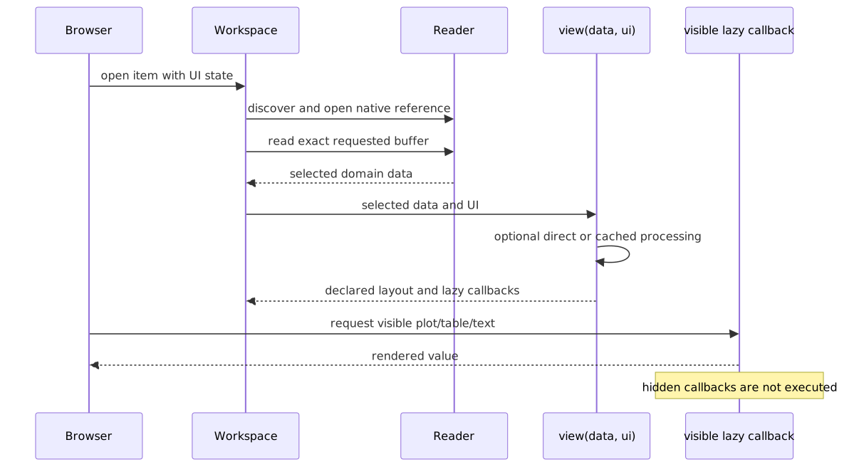
The author returns one Workspace. A reusable Reader handles discovery and
exact buffering; one unrestricted view(data, ui) callback does everything
after that.
Sigvue is intended to make signal viewing and repeatable batch processing simple to start and straightforward to extend. The same domain reader, processing functions, and plots work headlessly; the workspace adds discovery, buffer controls, lazy views, and optional durable batch actions without forcing the scientific pipeline into framework-specific stages.
Two standalone applications show the same core serving very different signal workflows:
- NOAA NEXRAD Viewer discovers Level III radar sequences, provides segmented scan playback, and renders full-resolution GIFs as durable batch results.
- SigMF Viewer discovers recordings and collections, reads exact moving windows, presents progressive waterfalls, and renders high-resolution per-channel PNGs in batch mode.
Install and run
python -m pip install sigvue
sigvue --config browser.toml
Open http://127.0.0.1:8000.
Application packages that provide a native pywebview window can install the shared desktop toolchain from a source checkout:
python -m pip install -e ".[desktop]"
The API

There is one application object:
Workspace(
    identifier="my-data",
    name="My Data",
    description="Inspect recordings.",
    reader=reader,
    view=view,
)
Inside view, the author decides what is shared, what is deferred, and whether
processing and plotting are separate at all.
Minimal file-backed workspace
from pathlib import Path

import plotly.graph_objects as go

from sigvue import Files, Workspace


def open_samples(path: Path) -> tuple[float, ...]:
    return tuple(float(value) for value in path.read_text().split(","))


def view(samples, ui):
    gain = float(ui.number("gain", default=2.0, minimum=0.0))
    values = tuple(value * gain for value in samples)

    ui.stat("Samples", len(samples))
    with ui.tab("Values"):
        ui.plot(
            lambda: go.Figure(go.Scatter(y=values)),
            key="values",
        )


def create_workspace(config=None):
    return Workspace(
        identifier="values",
        name="Values",
        description="Inspect sample files.",
        reader=Files("data", "*.samples", open_samples),
        view=view,
    )
There is no framework boundary between multiplication and plotting. The callback can call one combined function just as easily:
def view(samples, ui):
    with ui.tab("Values"):
        ui.plot(lambda: process_and_plot(samples), key="values")
That lambda is lazy. Hidden tabs and switcher choices are not executed.
Headless data access
Reader.discover() returns native author-owned references. Paths stay Path
objects; grouped collections and database keys stay domain objects.
reader = Files("data", "*.samples", open_samples)
path = reader.discover()[0]
samples = reader.load(path)
figure = process_and_plot(samples)
The same reader used by the browser is useful in scripts, notebooks, tests, and batch jobs.
Windowed data
reader = Files(root, "*.bin", open_recording).windowed(
    read_window,  # read_window(recording, start, stop)
    duration=lambda recording: recording.duration_seconds,
    default=0.100,
    minimum=0.010,
    step=0.010,
    overview=power_overview,
    overview_heatmap=low_resolution_waterfall,
    overview_colormap_control="colormap",
    overview_limits_control="dbfs_limits",
    overview_label="Median power",
)
Headlessly:
window = reader.load(path, start=2.0, stop=2.1)
Opened recordings, recent exact buffers, and overviews are revision-aware
cached for repeated browser requests. Reader buffering never approximates
scientific data. overview remains the lightweight line drawn across the
window bar; overview_heatmap optionally adds a rectangular numeric raster
behind it without changing the bar's geometry. Heatmap columns run
left-to-right in recording-time order and rows run bottom-to-top, so a
conventional frequency-x/time-y waterfall should be transposed before it is
supplied. The bar's expand icon selects the complete recording extent on
demand. The optional control bindings make the compact heatmap follow an
existing ui.colormap() picker and ui.limits() dBFS range; changing either
redraws the bar and the main plot together.
Segmented data
from sigvue import Segment

reader = Files(root, "*.json", open_collection).segmented(
    read_segment,  # read_segment(collection, selected_segment)
    duration=lambda collection: collection.duration,
    segments=lambda collection: tuple(
        Segment(event.id, event.start, event.duration, event.label)
        for event in collection.events
    ),
)
The callback receives the selected Segment, so irregular events and scans
retain their identity.
Seek and live playback
reader = Files(root, "*.bin", open_recording).playback(
    read_window,
    duration=lambda recording: recording.duration_seconds,
    default=0.020,
    minimum=0.001,
    maximum=0.100,
    buffer_step=0.001,
    mode="live",
    seek_step=0.010,
    refresh_interval=1.0,
)
This supplies an exact moving buffer. When maximum is given, the browser also
exposes its width.
Application-specific buffering
If a domain needs coupled controls that do not fit the regular helpers, the reader boundary stays open:
reader = Files(root, "*.collection", open_collection).buffered(
    read_buffer,       # ordinary headless read(opened, ...)
    select_buffer,     # select_buffer(opened, ui)
)
reader.load(reference, ...) calls read_buffer directly. The browser calls
select_buffer, which may declare buffer controls and then use that same exact
read. This does not introduce another processing or presentation stage.
Processing, caching, and lazy work
Sigvue does not decide how the callback is divided.
Direct processing is ordinary Python:
def view(data, ui):
    threshold = float(ui.number("threshold", default=3.0))
    events = detect_events(data, threshold)
    with ui.tab("Events"):
        ui.plot(lambda: plot_events(data, events), key="events")
For shared expensive work, ui.compute is an optional generic cache:
def view(data, ui):
    threshold = float(ui.number("threshold", default=3.0))
    events = ui.compute(
        "event-detection",
        lambda: detect_events(data, threshold),
    )
    with ui.tab("Events"):
        ui.plot(lambda: plot_events(data, events), key="events")
    with ui.tab("Table"):
        ui.table(lambda: event_rows(events), key="event-table")
By default, the cache key includes:
- the reader/source revision;
- the selected window, segment, or playback position;
- every control declared before
ui.compute.
The author may specify depends_on=(...) to narrow control dependencies, or
ignore ui.compute entirely.
Slow work needed by only one view belongs inside that view:
def view(data, ui):
    with ui.tab("Overview"):
        ui.plot(lambda: plot_overview(data), key="overview")

    with ui.tab("Slow diagnostics"):
        ui.plot(
            lambda: analyze_and_plot_diagnostics(data),
            key="diagnostics",
        )
Opening Overview does not run the diagnostics.
Exact complex layouts
The same callback supports all current layouts without another abstraction:
def view(data, ui):
    reference = str(ui.select(
        "phase_reference",
        default="Channel 1",
        options=channel_names(data),
    ))
    calibrated = ui.compute(
        "calibrated-radar",
        lambda: calibrate(data, phase_reference=reference),
    )

    ui.stat("Channels", calibrated.channel_count)

    with ui.tab("Waterfall"):
        ui.view_switcher(
            ("Domain", "Channel"),
            waterfall_views(calibrated, ui),
            key="waterfall-domain",
            selector=("buttons", "dropdown"),
            axis_navigation="bounded",
        )

    with ui.tab("Calibration", columns=(1, 1)):
        ui.plot(lambda: phase_plot(calibrated), key="phase")
        ui.table(calibrated.calibration_rows, key="calibration")
Tabs, weighted grids, nested groups, multidimensional switchers, display
controls, inline processing controls, tables, text, and deferred plots all stay
in the one nested ui API.
Custom discovery metadata
Paths receive useful defaults. Custom references may provide describe:
from sigvue import DataResource, Reader

reader = Reader(
    discover=discover_sequences,
    open=open_sequence,
    describe=lambda sequence: DataResource(
        identifier=sequence.id,
        title=sequence.title,
        source=sequence,
        timestamp=sequence.timestamp,
        tags=("radar", sequence.station),
        summary={"scan_count": sequence.scan_count},
    ),
)
Optional DiscoveryColumn values on Workspace define typed catalog columns.
Recursive readers preserve their relative directories as browser folders by
default. Set flatten_discovery=True on Workspace to show every discovered
item at the workspace root without changing its identifier, source, or reader.
Optional capabilities
Annotation, export, and batch support remain independent:
Workspace(
    ...,
    reader=reader,
    view=view,
    annotator=MyAnnotator(),
    exporter=MyExporter(),
    batch=MyBatchActions(),
    discovery_columns=MY_COLUMNS,
)
These contracts are imported directly from sigvue. Format-specific readers
and capabilities belong with the application or examples, not in Sigvue core.
Batch actions run independently of the current browser route. The notification
bell shows queued and running actions, follows them while the user browses other
workspaces or views, and retains their completed outputs for opening or path
copying. Reloading the page reconnects to jobs still owned by the server.

Configuration
A package exposes create_workspace(config):
[project.entry-points."sigvue.workspaces"]
my-analysis = "my_package.sigvue:create_workspace"
browser.toml chooses instances:
[browser]
title = "My data browser"

[[workspaces]]
use = "my-analysis"
id = "recordings"
name = "Recordings"
flatten_discovery = false

[workspaces.config]
data_root = "./data"
The profile is optional. Running sigvue without --config opens an empty
catalog with an Add workspace wizard. The wizard first discovers workspace
factories owned by the current project (including its browser.toml,
examples/browser.toml, and project entry points), falling back to installed
entry points only when the project has none. Selecting a different source
repository scopes discovery to that repository. The wizard pairs a factory
with a data directory and lets the user set the instance name,
identifier, description, category, tags, and additional factory
configuration. Flatten discovery can present all discovered items in one
list instead of retaining the reader's folder hierarchy. The new workspace
exists only in the running server unless
Save to a profile is selected; saving atomically creates or appends to the
chosen TOML file.
Applications can use the same profile-shaped spec without creating a file:
from pathlib import Path

from sigvue import create_app, workspace_launch_spec

workspace = workspace_launch_spec(
    {
        "use": "my-analysis",
        "id": "recordings",
        "name": "Recordings",
        "config": {"data_root": "./data"},
    },
    Path.cwd(),
)
app = create_app(workspace_specs=(workspace,))
app.configure_workspace(...) adds another instance later and optionally
accepts persist_path= to promote that session workspace to TOML. Profile
reloads preserve all other session-only workspaces.
The factory reads that location with
WorkspaceConfig(config).path("data_root"). The bundled examples deliberately
provide no code-level fallback, so browser.toml is their single source of
truth for data locations. The same factory may still be reused in several TOML
entries with different roots and metadata.
When a profile contains exactly one enabled workspace, the browser opens that
workspace's item discovery directly at /. Profiles with multiple workspaces
retain the searchable workspace catalog. Workspace code and configuration are
identical in both cases.
Runnable examples
Small examples live under examples/. The standalone examples
distribution covers communications, LTE waterfalls, calibrated multi-channel
radar, annotated ECG, weather radar, passive acoustics, seismology, stored
events, and native planetary data.
python -m pip install -e ".[examples]"
python -m examples.scripts.generate_all
sigvue --config examples/browser.toml
PyPI documentation
PyPI does not render Mermaid. The release workflow renders the diagrams:
python scripts/build_pypi_readme.py --ref "v$VERSION"
scripts/puppeteer-ci.json supplies Chromium's CI sandbox arguments.
Development
python -m pip install -e ".[test,release]"
python -m pytest -q
python -m build
python -m twine check dist/*
1 maintainer

Download files
Download the file for your platform. If you're not sure which to choose, learn more about installing packages.
Source Distribution
Built Distribution
Filter files by name, interpreter, ABI, and platform.
If you're not sure about the file name format, learn more about wheel file names.
Copy a direct link to the current filters
File details
Details for the file sigvue-2026.55.tar.gz.
File metadata
- Download URL: sigvue-2026.55.tar.gz
- Upload date:
- Size: 140.2 kB
- Tags: Source
- Uploaded using Trusted Publishing? No
- Uploaded via:
twine/6.1.0 CPython/3.13.14
File hashes
| Algorithm | Hash digest | |
|---|---|---|
| SHA256 |
639c1034954a04748ab55c612d29954b621a11d8c76ce86ddba9af082791652f
|
|
| MD5 |
a6ccfff05aca86fbba30cabed142b20c
|
|
| BLAKE2b-256 |
acaa5864417db6d7a48e4f020bbe4726b7a37d3fbc1fae6c0ea5ace83c968d20
|
File details
Details for the file sigvue-2026.55-py3-none-any.whl.
File metadata
- Download URL: sigvue-2026.55-py3-none-any.whl
- Upload date:
- Size: 110.7 kB
- Tags: Python 3
- Uploaded using Trusted Publishing? No
- Uploaded via:
twine/6.1.0 CPython/3.13.14
File hashes
| Algorithm | Hash digest | |
|---|---|---|
| SHA256 |
f6c358487bf63f022c9591733c18e8fbc3cf58c0e9eecbbc0ed6f573b2774084
|
|
| MD5 |
6bba66d5f5e59b85cb335c444cb86e8d
|
|
| BLAKE2b-256 |
7713325271a50020e0c670f51433fe3ad570fd33e2d3ebc5c579711d392287c7
|














