Compute technical indicators and build trade strategies in a simple way

Project description
simple-trade


simple-trade is a Python package for downloading market data, computing 100+ technical indicators, and backtesting trading strategies with ease. Build, backtest, and optimize your own trading strategies—or choose from 100+ premade trading strategies—without extra boilerplate.
Why simple-trade
- 100+ built-in indicators spanning trend, momentum, volume, and volatility.
- Plug-and-play 100+ premade trading strategies plus tools for custom strategy design.
- Integrated backtesting and optimization, and signal-combining tools in one package.
- Unified plotting, metrics, and reporting so results are easy to compare and share.
Features
- Data Fetching: Easily download historical stock data using
yfinance. - Technical Indicators: Compute more than 100+ technical indicators such as:
- Trend (e.g., MACD, ADX)
- Momentum (e.g., RSI, Stochastics)
- Volatility (e.g., Bollinger Bands, ATR)
- Volume (e.g., On-Balance Volume)
- Trading Strategies: Implement custom trading strategies or select from 100+ premade ones.
- Backtesting: Evaluate the performance of your trading strategies on historical data.
- Optimization: Optimize strategy parameters using techniques like grid search.
- Plotting: Visualize data, indicators, and backtest results using
matplotlib. - Combining: Combine different strategies to create more complex strategies.
Installation
Python
pip install simple-trade
or
python -m pip install simple-trade
QuickStart
Compute a technical indicator in just three lines of code.
from simple_trade import download_data, compute_indicator
data = download_data('TSLA', '2024-01-01', '2025-01-01', '1d')
data, columns, _ = compute_indicator(data, 'adx')
Choose, backtest, and optimize a premade strategy in just six lines of code.
from simple_trade import download_data, run_premade_trade, premade_optimizer
data = download_data('TSLA', '2024-01-01', '2025-01-01', '1d')
param_grid = {'short_window': [10, 20, 30], 'long_window': [50, 100, 150]}
_, best_results, _ = premade_optimizer(data, 'sma', param_grid)
sma_params = {'short_window': best_results['short_window'], 'long_window': best_results['long_window']}
sma_results, sma_portfolio, _ = run_premade_trade(data, "sma", sma_params)
Basic Usage
Table of Contents for Code Snippets
Calculate Indicators
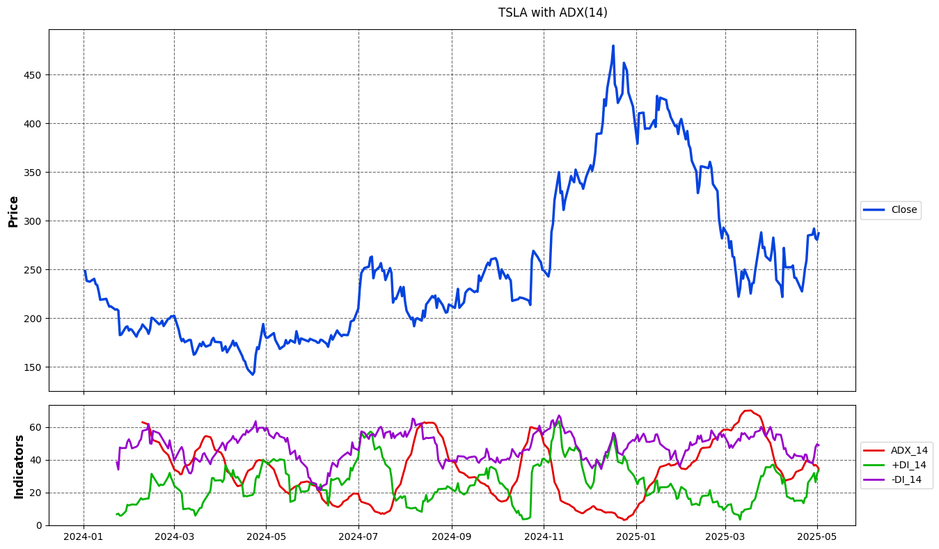
Use download_data function to download data using yfinance and use compute_indicator function to compute a technical indicator.
# Example for downloading data and computing a technical indicator

# Load packages and functions
from simple_trade import compute_indicator, download_data
from simple_trade import list_indicators

# Step 1: Download data
symbol = 'TSLA'
start = '2024-01-01'
end = '2025-01-01'
interval = '1d'
print(f"\nDownloading data for {symbol}...")
data = download_data(symbol, start, end, interval=interval)

# Step 2: Calculate indicator
parameters = dict()
columns = dict()
parameters["window"] = 14
data, columns, fig = compute_indicator(
    data=data,
    indicator='adx',
    parameters=parameters
)

# Step 3: Display result
fig.show()
Plot of Results
To see a list of all indicators, use list_indicators() function.
Backtesting Strategies
Use the run_premade_trade function to select from premade strategies or create your custom strategies using run_cross_trade/run_band_trade functions.
# Example for backtesting a premade strategy

# Load packages and functions
from simple_trade import download_data
from simple_trade import run_premade_trade
from simple_trade import list_premade_strategies
from simple_trade import print_results

# Step 1: Download data
symbol = 'AAPL'
start_date = '2020-01-01'
end_date = '2022-12-31'
interval = '1d'
data = download_data(symbol, start_date, end_date, interval=interval)

# Step 2: Set global parameters
global_parameters = {
    'initial_cash': 10000,
    'commission_long': 0.001,
    'commission_short': 0.001,
    'short_borrow_fee_inc_rate': 0.0,
    'long_borrow_fee_inc_rate': 0.0,
    'trading_type': 'long',
    'day1_position': 'none',
    'risk_free_rate': 0.0,
}

# Step 3: Set strategy parameters
strategy_name = 'sma'
specific_parameters = {
    'short_window': 25,
    'long_window': 75,
    'fig_control': 1,
}

# Step 4: Run backtest
parameters = {**global_parameters, **specific_parameters}
results, portfolio, fig = run_premade_trade(data, strategy_name, parameters)

# Step 5: Display and print results
fig.show()
print_results(results)
Plot of Results
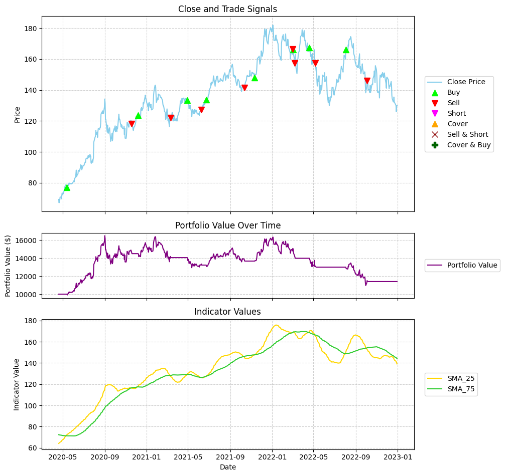
Print of Results
============================================================

🗓️ BACKTEST PERIOD:
  • Period: 2020-04-20 to 2022-12-30
  • Duration: 984 days
  • Trading Periods: 682

📊 BASIC METRICS:
  • Initial Investment: $10,000.00
  • Final Portfolio Value: $13,199.32
  • Total Return: 31.99%
  • Annualized Return: 10.80%
  • Number of Trades: 16
  • Total Commissions: $237.12

📈 BENCHMARK COMPARISON:
  • Benchmark Return: 87.48%
  • Benchmark Final Value: $18,748.45
  • Strategy vs Benchmark: -55.49%

📉 RISK METRICS:
  • Sharpe Ratio: 0.530
  • Sortino Ratio: 0.500
  • Maximum Drawdown: -32.50%
  • Average Drawdown: -14.25%
  • Max Drawdown Duration: 360 days
  • Avg Drawdown Duration: 43.43 days
  • Annualized Volatility: 25.89%

============================================================
To see a list of all premade strategies, use list_premade_strategies() function.
Optimizing Strategies
Use the premade_optimizer function to find the best parameters for your premade strategies or optimize your custom strategies using custom_optimizer function.
# Example for optimizing a premade strategy

# Load packages and functions
from simple_trade import download_data
from simple_trade import premade_optimizer

# Step 1: Load data
ticker = "AAPL"
start_date = "2020-01-01"
end_date = "2023-12-31"

data = download_data(ticker, start_date, end_date)

# Step 2: Load optimization parameters
# Define the parameter grid to search
param_grid = {
    'short_window': [10, 20, 30],
    'long_window': [50, 100, 150],
}

# Step 3: Set base parameters
base_params = {
    'initial_cash': 100000.0,
    'commission_long': 0.001,         # 0.1% commission
    'commission_short': 0.001,
    'trading_type': 'long',           # Only long trades
    'day1_position': 'none',
    'risk_free_rate': 0.02,
    'metric': 'total_return_pct',     # Metric to optimize
    'maximize': True,                 # Maximize the metric
    'parallel': False,                # Sequential execution for this example
    'fig_control': 0                  # No plotting during optimization
}

# Step 4: Run optimization
best_results, best_params, all_results = premade_optimizer(
    data=data,
    strategy_name='sma',
    parameters=base_params,
    param_grid=param_grid
)

# Step 5: Show top 3 parameter combinations
print("\nTop 3 SMA Parameter Combinations:")
sorted_results = sorted(all_results, key=lambda x: x['score'], reverse=True)
for i, result in enumerate(sorted_results[:3]):
    print(f"  {i+1}. {result['params']} -> {result['score']:.2f}%")
Output of Results
Top 3 SMA Parameter Combinations:
  1. {'short_window': 10, 'long_window': 50} -> 99.87%
  2. {'short_window': 20, 'long_window': 50} -> 85.69%
  3. {'short_window': 30, 'long_window': 50} -> 67.08%
Combining Strategies
Use the run_combined_trade function to combine multiple strategies.
# Example for combining premade strategies

# Load packages and functions
from simple_trade import download_data
from simple_trade import run_premade_trade
from simple_trade import run_combined_trade

# Step 1: Download data
print("Downloading stock data...")
symbol = 'AAPL'
start_date = '2020-01-01'
end_date = '2022-12-31'
interval = '1d'
data = download_data(symbol, start_date, end_date, interval=interval)

# Step 2: Set global parameters
global_parameters = {
    'initial_cash': 10000,
    'commission_long': 0.001,
    'commission_short': 0.001,
    'short_borrow_fee_inc_rate': 0.0,
    'long_borrow_fee_inc_rate': 0.0,
    'trading_type': 'long',
    'day1_position': 'none',
    'risk_free_rate': 0.0,
}

# Step 3: Compute RSI strategy
rsi_params = {
    'window': 14,
    'upper': 70,
    'lower': 30,
    'fig_control': 0
}

rsi_params = {**global_parameters, **rsi_params}
rsi_results, rsi_portfolio, _ = run_premade_trade(data, "rsi", rsi_params)

# Step 4: Compute SMA strategy
sma_params = {
    'short_window': 20,
    'long_window': 50,
    'fig_control': 0
}

sma_params = {**global_parameters, **sma_params}
sma_results, sma_portfolio, _ = run_premade_trade(data, "sma", sma_params)

# Step 5: Combine RSI and SMA strategies
strategies = {
    'RSI': {'results': rsi_results, 'portfolio': rsi_portfolio},
    'SMA': {'results': sma_results, 'portfolio': sma_portfolio}
}
combined_results, combined_portfolio, _ = run_combined_trade(
    portfolio_dfs=[rsi_portfolio, sma_portfolio],
    price_data=data,
    price_col='Close',
    combination_logic='majority',
    trading_type='long',
    fig_control=0,
    strategies=strategies,
    strategy_name='Majority',
    initial_cash=200,
    commission_long=0.001,
    commission_short=0.001
)

# Step 6: Show results
print(f"2 Trading Strategy Combination - Final Value: ${combined_results['final_value']:.2f}")
print(f"2 Trading Strategy Combination - Total Return: {combined_results['total_return_pct']}%")
print(f"2 Trading Strategy Combination - Number of Trades: {combined_results['num_trades']}")
print(f"2 Trading Strategy Combination - Sharpe Ratio: {combined_results['sharpe_ratio']:.3f}")
Output of Results
2 Trading Strategy Combination - Final Value: $318.11
2 Trading Strategy Combination - Total Return: 59.16%
2 Trading Strategy Combination - Number of Trades: 13
2 Trading Strategy Combination - Sharpe Ratio: 0.780
Examples
For more detailed examples, please refer to the Jupyter notebooks in the /examples directory:
/examples/indicators: Demonstrations of various technical indicators./examples/backtest: Examples of backtesting different strategies./examples/optimize: Examples of optimizing strategy parameters./examples/combine_trade: Examples of combining different strategies./examples/lists: Examples of listing functions.
Contributing
Contributions are welcome! Please feel free to submit a pull request or open an issue. (Further details can be added here if needed).
License
This project is licensed under the AGPL-3.0 License - see the LICENSE file for details.
Release history Release notifications | RSS feed


Download files
Download the file for your platform. If you're not sure which to choose, learn more about installing packages.
Source Distribution
Built Distribution
Filter files by name, interpreter, ABI, and platform.
If you're not sure about the file name format, learn more about wheel file names.
Copy a direct link to the current filters
File details
Details for the file simple_trade-0.3.4.tar.gz.
File metadata
- Download URL: simple_trade-0.3.4.tar.gz
- Upload date:
- Size: 238.8 kB
- Tags: Source
- Uploaded using Trusted Publishing? No
- Uploaded via: twine/6.2.0 CPython/3.11.4
File hashes
| Algorithm | Hash digest | |
|---|---|---|
| SHA256 |
07fed07db855473249f6344f99947ad15905fea077097800091b073d9176f587
|
|
| MD5 |
2d1a58b0c62b94fbac8c421a123c6a88
|
|
| BLAKE2b-256 |
2da60015b672302cfb544aee589688f154d673af02f96f6d19f16f3954279fd7
|
File details
Details for the file simple_trade-0.3.4-py3-none-any.whl.
File metadata
- Download URL: simple_trade-0.3.4-py3-none-any.whl
- Upload date:
- Size: 350.8 kB
- Tags: Python 3
- Uploaded using Trusted Publishing? No
- Uploaded via: twine/6.2.0 CPython/3.11.4
File hashes
| Algorithm | Hash digest | |
|---|---|---|
| SHA256 |
019798b162788eb25d18076c9a426748313a13f62b2da333cdf1c532f814efe0
|
|
| MD5 |
352902238a3b290286275d188e043b86
|
|
| BLAKE2b-256 |
be0e90df8e8526e160fffdd8712328c34eaa8336fa53cbe1ea93048295417f06
|


