Compute technical indicators and build trade strategies in a simple way

Project description
simple-trade


A Python library that allows you to compute technical indicators and build trade strategies in a simple way.
Features
- Data Fetching: Easily download historical stock data using
yfinance. - Technical Indicators: Compute a variety of technical indicators:
- Trend (e.g., Moving Averages, MACD, ADX)
- Momentum (e.g., RSI, Stochastics)
- Volatility (e.g., Bollinger Bands, ATR)
- Volume (e.g., On-Balance Volume)
- Trading Strategies: Implement and backtest common trading strategies:
- Cross Trade Strategies (
cross_trade) - Band Trading Strategies (
band_trade)
- Cross Trade Strategies (
- Backtesting: Evaluate the performance of your trading strategies on historical data.
- Optimization: Optimize strategy parameters using techniques like grid search.
- Plotting: Visualize data, indicators, and backtest results using
matplotlib.
Installation
- Clone the repository:
git clone <repository_url> # Replace with your repo URL
cd simple-trade
- Create and activate a virtual environment (recommended):
python -m venv myenv
# On Windows
myenv\Scripts\activate
# On macOS/Linux
source myenv/bin/activate
- Install the package and dependencies:
pip install .
Alternatively, installed with PyPI:pip install simple-trade
Dependencies
- Python >= 3.10
- yfinance
- pandas
- numpy
- joblib
- matplotlib
These will be installed automatically when you install simple-trade using pip.
Basic Usage
Here's a quick example of how to download data and compute a technical indicator:
# Load Packages and Functions
import pandas as pd
from simple_trade import compute_indicator, download_data
from simple_trade import IndicatorPlotter
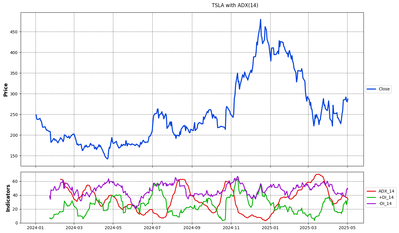
# Step 1: Download data
symbol = 'TSLA'
start = '2024-01-01'
end = '2025-01-01'
interval = '1d'
print(f"\nDownloading data for {symbol}...")
data = download_data(symbol, start, end, interval=interval)
# Step 2: Calculate indicator
parameters = dict()
columns = dict()
parameters["window"] = 14
columns["high_col"] = 'High'
columns["low_col"] = 'Low'
columns["close_col"] = 'Close'
data = compute_indicator(
data=data,
indicator='adx',
parameters=parameters,
columns=columns
)
# Step 3: Plot the indicator
plotter = IndicatorPlotter()
window = parameters["window"]
columns = [f'ADX_{window}', f'+DI_{window}', f'-DI_{window}']
fig = plotter.plot_results(
data,
price_col='Close',
column_names=columns,
plot_on_subplot=True,
title=f"{symbol} with ADX({window})"
)
# Step 4: Display the plot
fig.show()
Plot of Results
Advanced Usage
Backtesting Strategies
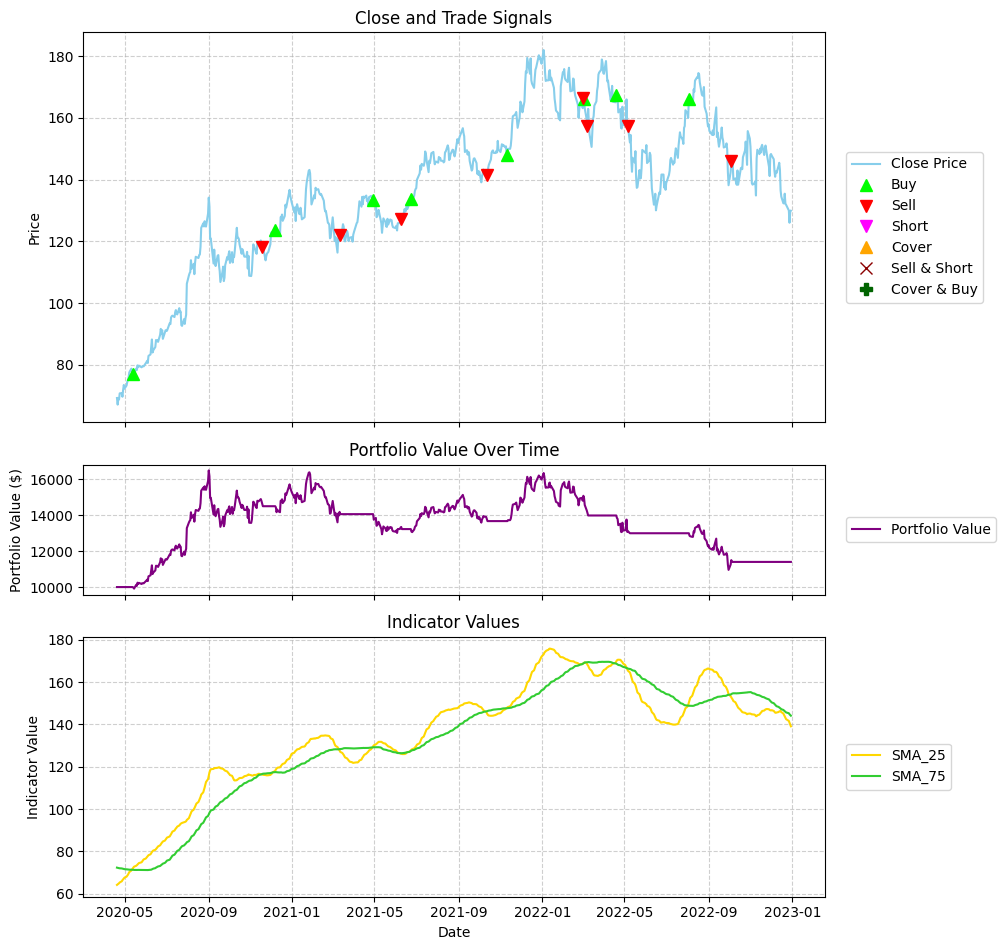
Use the backtesting module to simulate strategies like moving average crossovers (cross_trade) or Bollinger Band breakouts (band_trade).
# Load Packages and Functions
import pandas as pd
from simple_trade import download_data, compute_indicator
from simple_trade import CrossTradeBacktester
from simple_trade import BacktestPlotter

# Step 1: Download data
symbol = 'AAPL'
start_date = '2020-01-01'
end_date = '2022-12-31'
interval = '1d'
data = download_data(symbol, start_date, end_date, interval=interval)

# Step 2: Download indicators
short_window = 25
long_window = 75
data = compute_indicator(data, indicator='sma', window=short_window)
data = compute_indicator(data, indicator='sma', window=long_window)

# Step 3: Initialize strategy
initial_cash = 10000.0
commission = 0.01
backtester = CrossTradeBacktester(initial_cash=initial_cash, commission_long=commission)

results, portfolio = backtester.run_cross_trade(
    data=data,
    short_window_indicator="SMA_25",
    long_window_indicator="SMA_75",
    price_col='Close',
)

# Step 4: Produce results
backtester.print_results(results)

# Step 5: Plot results
plotter = BacktestPlotter()
indicator_cols_to_plot = [f'SMA_{short_window}', f'SMA_{long_window}']
fig = plotter.plot_results(
    data_df=data,
    history_df=portfolio,
    price_col='Close',
    indicator_cols=indicator_cols_to_plot,
    title=f"Cross Trade (Long Only) (SMA-{short_window} vs SMA-{long_window})"
)

# Step 6: Display the plot
plt.show()
Output of Results
============================================================
              ✨ Cross Trade (SMA_25/SMA_75) ✨
============================================================

🗓️ BACKTEST PERIOD:
  • Period: 2020-04-20 to 2022-12-30
  • Duration: 984 days
  • Trading Days: 682

📊 BASIC METRICS:
  • Initial Investment: $10,000.00
  • Final Portfolio Value: $11,400.77
  • Total Return: 14.01%
  • Annualized Return: 4.96%
  • Number of Trades: 16
  • Total Commissions: $1,936.74

📈 BENCHMARK COMPARISON:
  • Benchmark Return: 71.32%
  • Benchmark Final Value: $17,132.49
  • Strategy vs Benchmark: -57.31%

📉 RISK METRICS:
  • Sharpe Ratio: 0.320
  • Sortino Ratio: 0.260
  • Maximum Drawdown: -33.59%
  • Average Drawdown: -15.36%
  • Max Drawdown Duration: 849 days
  • Avg Drawdown Duration: 61.33 days
  • Annualized Volatility: 23.75%
Plot of Results
Optimizing Strategies
The optimizer module allows you to find the best parameters for your strategy (e.g., optimal moving average windows).
# Load Packages and Functions
from simple_trade import download_data, compute_indicator
from simple_trade import CrossTradeBacktester
from simple_trade import Optimizer

# Step 1: Load Data
ticker = "AAPL"
start_date = "2020-01-01"
end_date = "2023-12-31"

data = download_data(ticker, start_date, end_date)

# Step 2: Load Optimization Parameters
# Define the parameter grid to search
param_grid = {
    'short_window': [10, 20, 30],
    'long_window': [50, 100, 150],
}
# Define constant parameters for the backtester
initial_capital = 100000
commission_fee = 0.001 # 0.1%
constant_params = {
    'initial_cash': initial_capital,
    'commission_long': commission_fee,
    'price_col': 'Close'
}
# Define the metric to optimize and whether to maximize or minimize
metric_to_optimize = 'total_return_pct'
maximize_metric = True

# Step 3: Define the wrapper function
def run_cross_trade_with_windows(data, short_window, long_window, **kwargs):
    # Work on a copy of the data
    df = data.copy()

    # Compute the SMA indicators
    df = compute_indicator(df, indicator='sma', parameters={'window': short_window}, columns={'close_col': 'Close'})
    df = compute_indicator(df, indicator='sma', parameters={'window': long_window}, columns={'close_col': 'Close'})

    # Get the indicator column names
    short_window_indicator = f"SMA_{short_window}"
    long_window_indicator = f"SMA_{long_window}"

    # Create a backtester instance
    backtester = CrossTradeBacktester(
        initial_cash=kwargs.pop('initial_cash', 10000),
        commission_long=kwargs.pop('commission_long', 0.001),
    )

    # Run the backtest
    return backtester.run_cross_trade(
        data=df,
        short_window_indicator=short_window_indicator,
        long_window_indicator=long_window_indicator,
        **kwargs
    )

# Step 4: Instantiate and Run Optimizer
print("Initializing Optimizer...")
optimizer = Optimizer(
    data=data,
    backtest_func=run_cross_trade_with_windows,  # Use our wrapper function
    param_grid=param_grid,
    metric_to_optimize=metric_to_optimize,
    maximize_metric=maximize_metric,
    constant_params=constant_params
)

print("\nRunning Optimization (Parallel)...")
# Run optimization with parallel processing (adjust n_jobs as needed)
results = optimizer.optimize(parallel=True, n_jobs=-1) # n_jobs=-1 uses all available cores

# --- Display Results ---
print("\n--- Optimization Results ---")

# Unpack results
best_params, best_metric_value, all_results = results

print("\n--- Top 5 Parameter Combinations ---")
# Sort results for display
sorted_results = sorted(all_results, key=lambda x: x[1], reverse=maximize_metric)
for i, (params, metric_val) in enumerate(sorted_results[:5]):
    print(f"{i+1}. Params: {params}, Metric: {metric_val:.4f}")
Output of Results
print("\nRunning Optimization (Parallel)...")
# Run optimization with parallel processing (adjust n_jobs as needed)
results = optimizer.optimize(parallel=True, n_jobs=-1) # n_jobs=-1 uses all available cores

# --- Display Results ---
print("\n--- Optimization Results ---")

# Unpack results
best_params, best_metric_value, all_results = results

print("\n--- Top 5 Parameter Combinations ---")
# Sort results for display
sorted_results = sorted(all_results, key=lambda x: x[1], reverse=maximize_metric)
for i, (params, metric_val) in enumerate(sorted_results[:5]):
    print(f"{i+1}. Params: {params}, Metric: {metric_val:.4f}")

Initializing Optimizer...
Generated 9 parameter combinations.

Running Optimization (Parallel)...
Starting optimization for 9 combinations...
Metric: total_return_pct (Maximize) | Parallel: True (n_jobs=-1)
Using 16 parallel jobs.
[Parallel(n_jobs=16)]: Using backend LokyBackend with 16 concurrent workers.
[Parallel(n_jobs=16)]: Done   2 out of   9 | elapsed:    9.0s remaining:   31.6s
[Parallel(n_jobs=16)]: Done   4 out of   9 | elapsed:    9.4s remaining:   11.7s
[Parallel(n_jobs=16)]: Done   6 out of   9 | elapsed:    9.5s remaining:    4.7s
Optimization finished in 9.86 seconds.
Best Parameters found: {'short_window': 10, 'long_window': 50}
Best Metric Value (total_return_pct): 89.0500

--- Optimization Results ---

--- Top 5 Parameter Combinations ---
1. Params: {'short_window': 10, 'long_window': 50}, Metric: 89.0500
2. Params: {'short_window': 20, 'long_window': 50}, Metric: 76.6100
3. Params: {'short_window': 30, 'long_window': 50}, Metric: 60.6400
4. Params: {'short_window': 10, 'long_window': 150}, Metric: 19.4100
5. Params: {'short_window': 20, 'long_window': 100}, Metric: 10.9600
[Parallel(n_jobs=16)]: Done   9 out of   9 | elapsed:    9.7s finished
Examples
For more detailed examples, please refer to the Jupyter notebooks in the /examples directory:
/examples/indicators: Demonstrations of various technical indicators./examples/backtest: Examples of backtesting different strategies./examples/optimize: Examples of optimizing strategy parameters.
Contributing
Contributions are welcome! Please feel free to submit a pull request or open an issue. (Further details can be added here if needed).
License
This project is licensed under the AGPL-3.0 License - see the LICENSE file for details.
Release history Release notifications | RSS feed


Download files
Download the file for your platform. If you're not sure which to choose, learn more about installing packages.
Source Distribution
Built Distribution
Filter files by name, interpreter, ABI, and platform.
If you're not sure about the file name format, learn more about wheel file names.
Copy a direct link to the current filters
File details
Details for the file simple_trade-0.1.2.tar.gz.
File metadata
- Download URL: simple_trade-0.1.2.tar.gz
- Upload date:
- Size: 5.3 MB
- Tags: Source
- Uploaded using Trusted Publishing? No
- Uploaded via: twine/6.1.0 CPython/3.11.4
File hashes
| Algorithm | Hash digest | |
|---|---|---|
| SHA256 |
68f972265d194cf038cb7853cae6fb9871be9e3b51b4179a4d16f295313cc88c
|
|
| MD5 |
13b8b0c5c3e7cbaed25b040f9d97ab6f
|
|
| BLAKE2b-256 |
49028fa477cbf87943c38f88412e88e0669fe52fa5750a767e18373cf9ed2f5e
|
File details
Details for the file simple_trade-0.1.2-py3-none-any.whl.
File metadata
- Download URL: simple_trade-0.1.2-py3-none-any.whl
- Upload date:
- Size: 84.0 kB
- Tags: Python 3
- Uploaded using Trusted Publishing? No
- Uploaded via: twine/6.1.0 CPython/3.11.4
File hashes
| Algorithm | Hash digest | |
|---|---|---|
| SHA256 |
eda09ebfcf1e8254162aea5d8167da228b6296b2c8359cbdabc61af349f1c519
|
|
| MD5 |
866e9f096e88404ac43b139e4e510d1c
|
|
| BLAKE2b-256 |
20d3f7c4cfab1952e1b916c73824f029d75428dbc1d9d1f244cea1ccb5c20ff6
|


