






Given experimental data, it is often desirable to produce a function whose values match the data to some degree. This package implements a robust approach to data fitting based on the minimization problem
\|\lambda\Delta f\|^2_{L^2(\Omega)} + \sum_i (f(x_i) - y_i)^2 \to\min
(A similar idea is used in for data smoothing in signal processing; see, e.g., section 8.3 in this document.)
Unlike polynomial regression or Gauss-Newton, smoothfit makes no assumptions about the function other than that it is smooth.
The generality of the approach makes it suitable for function whose domain is multidimensional, too.
Pics or it didn't happen
Runge's example

Runge's example function is a tough nut for classical polynomial regression.
If there is no noise in the input data, the parameter lmbda can be chosen quite small
such that all data points are approximated well. Note that there are no oscillations in
the output function u.
import matplotlib.pyplot as plt
import numpy as np
import smoothfit

a = -1.5
b = +1.5

# plot original function
x = np.linspace(a, b, 201)
plt.plot(x, 1 / (1 + 25 * x ** 2), "-", color="0.8", label="1 / (1 + 25 * x**2)")

# sample points
x0 = np.linspace(-1.0, 1.0, 21)
y0 = 1 / (1 + 25 * x0 ** 2)
plt.plot(x0, y0, "xk")

# smoothfit
basis, coeffs = smoothfit.fit1d(x0, y0, a, b, 1000, degree=1, lmbda=1.0e-6)
plt.plot(basis.mesh.p[0], coeffs[basis.nodal_dofs[0]], "-", label="smooth fit")

plt.ylim(-0.1)
plt.grid()
plt.show()
Runge's example with noise

If the data is noisy, lmbda needs to be chosen more carefully. If too small, the
approximation tries to resolve all data points, resulting in many small oscillations.
If it's chosen too large, no details are resolved, not even those of the underlying
data.
import matplotlib.pyplot as plt
import numpy as np
import smoothfit

a = -1.5
b = +1.5

# plot original function
x = np.linspace(a, b, 201)
plt.plot(x, 1 / (1 + 25 * x ** 2), "-", color="0.8", label="1 / (1 + 25 * x**2)")

# 21 sample points
rng = np.random.default_rng(0)
n = 51
x0 = np.linspace(-1.0, 1.0, n)
y0 = 1 / (1 + 25 * x0 ** 2)
y0 += 1.0e-1 * (2 * rng.random(n) - 1)
plt.plot(x0, y0, "xk")

lmbda = 5.0e-2
basis, coeffs = smoothfit.fit1d(x0, y0, a, b, 1000, degree=1, lmbda=lmbda)
plt.plot(basis.mesh.p[0], coeffs[basis.nodal_dofs[0]], "-", label="smooth fit")

plt.grid()
plt.show()
Few samples
import numpy as np
import smoothfit

x0 = np.array([0.038, 0.194, 0.425, 0.626, 1.253, 2.500, 3.740])
y0 = np.array([0.050, 0.127, 0.094, 0.2122, 0.2729, 0.2665, 0.3317])
u = smoothfit.fit1d(x0, y0, 0, 4, 1000, degree=1, lmbda=1.0)
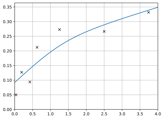
Some noisy example data taken from Wikipedia.
A two-dimensional example
import meshzoo
import numpy as np
import smoothfit

n = 200
rng = np.random.default_rng(123)
x0 = rng.random((n, 2)) - 0.5
y0 = np.cos(np.pi * np.sqrt(x0.T[0] ** 2 + x0.T[1] ** 2))

# create a triangle mesh for the square
points, cells = meshzoo.rectangle_tri(
    np.linspace(-1.0, 1.0, 32), np.linspace(-1.0, 1.0, 32)
)

basis, u = smoothfit.fit(x0, y0, points, cells, lmbda=1.0e-4, solver="dense-direct")

# Write the function to a file
basis.mesh.save("out.vtu", point_data={"u": u})
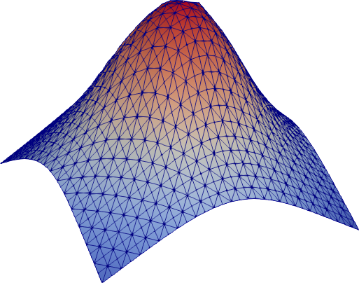
This example approximates a function from R2 to R (without noise in the
samples). Note that the absence of noise the data allows us to pick a rather small
lmbda such that all sample points are approximated well.
Comparison with other approaches
Polynomial fitting/regression

The classical approach to data fitting is polynomial regression. Polynomials are chosen because they are very simple, can be evaluated quickly, and can be made to fit any function very closely.
There are, however, some fundamental problems:
- Your data might not actually fit a polynomial of low degree.
- Runge's phenomenon.
This above plot highlights the problem with oscillations.
Fourier smoothing
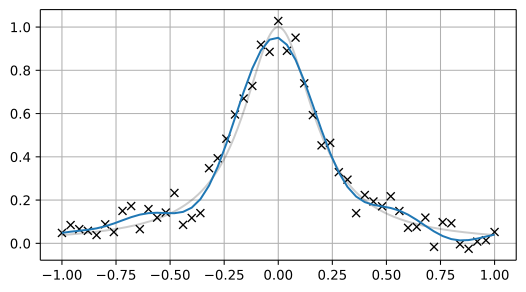
One approach to data fitting with smoothing is to create a function with all data points, and simply cut off the high frequencies after Fourier transformation.
This approach is fast, but only works for evenly spaced samples.
For equidistant curve fitting there is nothing else that could compete with the Fourier series. -- Cornelius Lanczos
import matplotlib.pyplot as plt
import numpy as np


rng = np.random.default_rng(0)

# original function
x0 = np.linspace(-1.0, 1.0, 1000)
y0 = 1 / (1 + 25 * x0 ** 2)
plt.plot(x0, y0, color="k", alpha=0.2)

# create sample points
n = 51
x1 = np.linspace(-1.0, 1.0, n)  # only works if samples are evenly spaced
y1 = 1 / (1 + 25 * x1 ** 2) + 1.0e-1 * (2 * rng.random(x1.shape[0]) - 1)
plt.plot(x1, y1, "xk")

# Cut off the high frequencies in the transformed space and transform back
X = np.fft.rfft(y1)
X[5:] = 0.0
y2 = np.fft.irfft(X, n)
#
plt.plot(x1, y2, "-", label="5 lowest frequencies")

plt.grid()
plt.show()
1 maintainer

Metadata
1 maintainer
Release files for smoothfit 0.4.1
For a detailed explanation of source distributions (sdists) and built distributions (wheels), please see the package formats documentation.
Built distribution (wheel)
| File | Interpreter | ABI | Platform | Reset |
|---|---|---|---|---|
| smoothfit-0.4.1-py3-none-any.whl | Python 3 | none | any | Details |
Release files / smoothfit-0.4.1-py3-none-any.whl
| Download URL | smoothfit-0.4.1-py3-none-any.whl |
|---|---|
| Size | 15.8 kB |
| Tags | Python 3 |
|
SHA-256 checksum How to use checksums |
928946c3b80791e28d3a26d0314c4ba20f747b63c94a0470f6fef7ea72873943
|
|
BLAKE2b-256 checksum How to use checksums |
f848a0e53c2f8a97f2189ba90596c26b33afbab40479258a9d21e3764aad094e
|
| Upload date | |
|
Uploaded using Trusted Publishing? What is trusted publishing? |
No |
| Uploaded via |
twine/4.0.1 CPython/3.11.2
|
Security for smoothfit 0.4.1
Provenance
Provenance describes where a file came from. On PyPI, provenance is shared via attestations, which provide a verifiable record of the build or publishing details. View details, limitations and caveats.
No provenance found
None of the files in this release were uploaded with provenance metadata.
A note on package security
PyPI is a repository for distributing packages, not a service for auditing them. While third-party security researchers and our staff do their best to detect and remove malicious packages, PyPI cannot guarantee the quality, security or suitability of any given package.
To learn more about protecting yourself from malicious actors, visit our package security documentation.














