

snp2le: S-Parameter To Lumped Element Netlist Converter






(c) 2026 Simon Dorrer
Institute for Integrated Circuits and Quantum Computing (IICQC), Johannes Kepler University (JKU), Linz, Austria
[!IMPORTANT] The converter (GUI and CLI) runs anywhere with Python ≥ 3.10, see Install below. Running the exported netlists in a testbench additionally needs Xschem plus Ngspice and/or VACASK. The easiest way to get all of them is the IIC-OSIC-TOOLS container. Since tag
2026.07,snp2lehas been installed directly in the IIC-OSIC-TOOLS container.
Description
snp2le turns a Touchstone .sNp S-parameter file (for example from an AWS Palace EM simulation) into an equivalent lumped-element netlist for Ngspice (Berkeley SPICE3) and VACASK (Spectre syntax). An EM-extracted structure can then be co-simulated at circuit level, without re-running the field solve.
It offers two conversion philosophies:
- Universal (any N-port). Vector-fits the S-parameters with scikit-rf
VectorFitting, optionally enforces passivity, and synthesises a passive macromodel of R, C and controlled sources. It works for any structure and port count, and is electrically exact but not physically interpretable. Its resistors are emitted noiseless (noisy=0, understood by both Ngspice and VACASK): they exist to reproduce the fitted response, not to model a device, and charging thermal noise against them would report noise that tracks the fit order instead of the structure. A noise budget through a universal model must account for the structure's real loss separately. - Structure-specific. Fits a known physical topology, so every component maps to reality (series L, shunt C, coupling k, and so on) at a chosen extraction frequency. Its resistors model real loss (a Wilkinson's isolation resistor, a coil's conductor loss), so they keep their thermal noise. See Available structures.
Either mode fits the file's full frequency range by default, or a fit range of your choosing (e.g. only 110 GHz to 170 GHz of a 80 GHz to 240 GHz EM sweep), so the model order is spent on the band the block actually operates in.
A single dialect-agnostic Circuit IR drives both netlist backends and the on-screen schematic, so the outputs always agree. The code is split into a pure-Python, Qt-free snp2le.core (fully unit-tested) and a thin snp2le.gui on PySide6-Essentials, both driven by one entry point, engine.convert(state, net).
A fit of a large N-port runs for seconds to minutes, so it runs on a worker thread and reports as it goes: the GUI shows what the fit is doing, how long it has been running and a progress bar, then leaves the outcome on screen when it finishes, and the CLI draws the same progress on a terminal. See Watching a conversion.
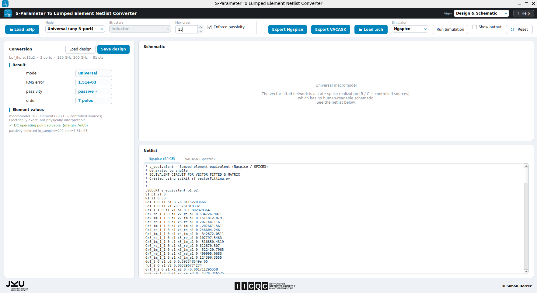
The snp2le GUI converting a band-pass filter (BPF) S-parameter file into a lumped-element netlist.
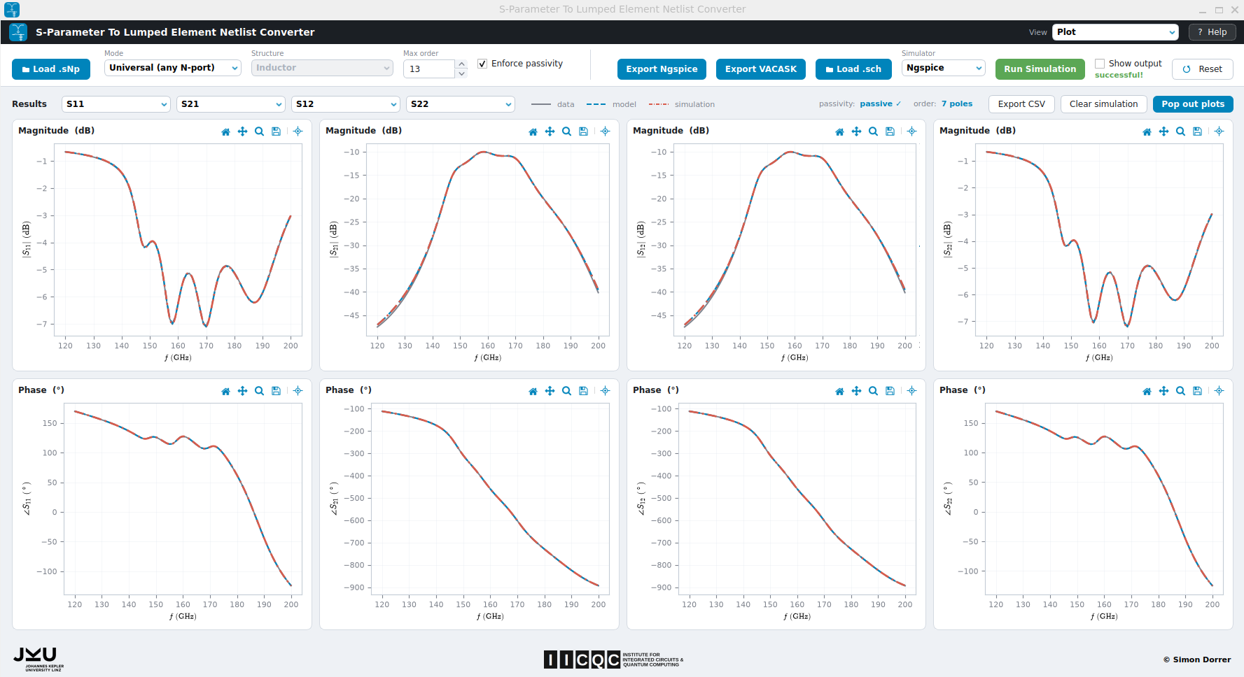
Plot view: loaded data (grey) vs extracted model (blue) vs imported testbench simulation (red).
Directory Structure
📁 snp2le/
├─ 📁 doc/                    architecture notes and screenshots
│  ├─ 📁 fig/                 GUI and plot screenshots
│  └─ architecture.md         data flow, internals, how to extend
├─ 📁 netlist/                exported lumped-element netlists
│  ├─ 📁 spectre/             VACASK (.inc) + syntax_cheatsheet.inc
│  └─ 📁 spice/               Ngspice (.spice)
├─ 📁 schematic/
│  └─ 📁 xschem/              DUT symbols (*.sym) and xschemrc
├─ 📁 snp2le/                 the application package (pip-installable)
│  ├─ 📁 core/                pure Python, Qt-free, all the maths
│  │  ├─ 📁 structures/       physical extractors, one per topology
│  │  │  ├─ __init__.py       registry (GUI dropdown + CLI find it)
│  │  │  ├─ base.py
│  │  │  ├─ balun.py
│  │  │  ├─ branchline.py
│  │  │  ├─ inductor_pi.py
│  │  │  ├─ mim_cap.py
│  │  │  ├─ tline.py
│  │  │  └─ wilkinson.py
│  │  ├─ __init__.py
│  │  ├─ dc.py                DC operating-point (singularity) check
│  │  ├─ engine.py            convert(state, net) -> Results, the entry point
│  │  ├─ io.py                load Touchstone, parse Ngspice tables
│  │  ├─ ir.py                dialect-agnostic Circuit IR
│  │  ├─ mna.py               rebuild N-port S-parameters from an RLC IR
│  │  ├─ netlist.py           render the IR to Ngspice and VACASK
│  │  ├─ progress.py          progress reporting for long conversions
│  │  ├─ state.py             ConverterState and Results dataclasses
│  │  ├─ units.py             engineering-notation parse and format
│  │  ├─ universal.py         vector-fit passive macromodel
│  │  └─ xschem.py            headless Xschem netlist and simulate
│  ├─ 📁 examples/            Touchstone .sNp samples (BPF, ind, balun, ...)
│  ├─ 📁 gui/                 PySide6-Essentials, no maths
│  │  ├─ 📁 assets/           logos (svg and png), snp2le.ico
│  │  ├─ __init__.py
│  │  ├─ design_view.py       results, values, tolerances, schematic
│  │  ├─ fit_runner.py        runs engine.convert on a worker thread
│  │  ├─ fit_status.py        the conversion progress / outcome indicator
│  │  ├─ main_window.py       the controller
│  │  ├─ plot_view.py         four S-parameter / extracted-param plots
│  │  ├─ top_bar.py           load, mode, structure, options, run
│  │  └─ ...                  help_dialog.py, style.py, widgets.py, and more
│  ├─ __init__.py             package version
│  ├─ __main__.py             single entry point (GUI, GUI on a file, or -b for the CLI)
│  ├─ app.py                  the GUI launcher (__main__ starts it)
│  └─ cli.py                  the batch CLI behind -b
├─ 📁 testbenches/
│  └─ 📁 xschem/              N-port testbenches (Ngspice and VACASK)
│     ├─ 📁 plot_simulations/ plot scripts (plot_*.py, sparam_plot.py, ngspice2python.py)
│     │  ├─ 📁 data/          simulation result tables, overlaid on the plots
│     │  └─ 📁 figures/       PNG figures written by the plot scripts
│     └─ 📁 simulations/      generated netlists and raw output (not tracked)
├─ 📁 tests/                  pytest suite
│  ├─ test_core.py
│  ├─ test_gui_fit_progress.py  headless non-blocking-conversion regressions
│  ├─ test_gui_fit_range.py   headless fit-range control
│  ├─ test_gui_launch_file.py  headless GUI opened on a command-line file
│  ├─ test_gui_passivity_ceiling.py  headless passivity-ceiling control
│  ├─ test_gui_sim_flow.py    headless GUI run/poll/import regressions
│  ├─ test_gui_top_bar_layout.py  headless control-strip layout invariants
│  ├─ test_gui_view_switch.py  headless View switch (both views on screen)
│  ├─ test_main_dispatch.py   the entry point's argument dispatch (no Qt)
│  ├─ test_progress.py        progress reporting and the fit watcher
│  ├─ test_qt_essentials.py   guards the Essentials-only dependency
│  ├─ test_reproducibility.py same input, same model, across processes
│  └─ test_xschem.py
├─ 📁 LICENSES/               license texts the REUSE check resolves against
│  └─ Apache-2.0.txt
├─ 📁 .github/workflows/      CI
│  └─ license-check.yml       reuse lint: every file carries copyright + license
├─ CITATION.cff
├─ LICENSE                    Apache-2.0
├─ MANIFEST.in                sdist manifest (bundles examples and assets)
├─ pyproject.toml             packaging, dependencies, snp2le entry point
├─ README.md
├─ REUSE.toml                 licensing of files that cannot carry an SPDX header
└─ requirements.txt           runtime dependencies (mirrors pyproject.toml)
How to Use
Install
From PyPI:
pip install snp2le
# or, for an isolated install with its own command on PATH:
pipx install snp2le
From source (for development), an editable install pulls in every dependency:
git clone https://github.com/iic-jku/snp2le.git
cd snp2le

python -m venv .venv
# Windows:        .venv\Scripts\activate
# macOS / Linux:  source .venv/bin/activate

pip install -e .
Run the GUI
snp2le              # after installing (pip / pipx)
snp2le design.s4p   # the same, opened on that Touchstone file
python -m snp2le    # from the repo root of a source checkout, no install needed
A bundled example is preloaded when no file is named. More live in snp2le/examples/.
Naming a .sNp file on the command line opens the GUI on it instead of the example, with the port count, the fit range and the first conversion taken from that file. This is how a tool that just wrote the file hands it over, for example the Model Fit button of setupEM after an AWS Palace run. Reset returns to that file rather than to the example. A file that cannot be read is reported in a dialog (and on stderr) and the example is loaded in its place, so the window opens either way.
[!NOTE] Start it as a module (
python -m snp2le), notpython snp2le/app.py. The launcher imports thesnp2lepackage, which Python only finds when it is run as a module from the repo root (or afterpip install).
Typical workflow
- Load a Touchstone
.sNpfile from the top bar, or name it on the command line (snp2le design.s4p, see above). The header shows the port count and frequency range. - Choose a mode. Universal (set Max order, Enforce passivity and the Passivity ceiling it works towards) or Structure-specific (pick a structure and set the extraction frequency). Some structures expose an extra option such as Stages, Isolation R or Resistive loss.
- Restrict the fit range (optional, both modes). The Fit range (GHz) fields start at the loaded file's own span, so they always name the band being fitted. Enter two plain numbers in GHz (e.g.
110and170) to fit only a sub-band. The Result panel shows the band actually fitted, and the RMS error, the tolerances, the plots and a testbench run's sweep all follow it. An edge outside the data is clamped to the data and reported, an empty or inverted band is refused. - Inspect the result, element values, per-element tolerances at the extraction frequency, the drawn schematic, and the generated netlist in the Design & Schematic view.
- Compare the loaded data (grey) against the extracted model (blue) in the Plot view (up to four traces, magnitude and phase). The View switch at the right of the title bar carries both views side by side and fills the one you are on, so a click moves between them.
- Export the netlist. Export Ngspice writes a
.spicefile and Export VACASK writes an.incfile. The.SUBCKTis named after the file, so a testbench that instantiates it resolves the include.
[!TIP] The Help button in the top bar opens a full in-app guide to every control.
Passivity and the passivity ceiling
A macromodel is passive when the largest singular value of its S-matrix, sigma_max, stays at or below 1 at every frequency. That is the same statement as "it can never deliver more power than it absorbs". A non-passive model is not merely inaccurate: a transient run can feed on the excess energy and grow without bound, so the simulation diverges or refuses to converge even though its AC response looked fine.
Making a model passive is not free. A vector fit typically violates passivity outside the band it was fitted to, and pushing it back below 1 there costs accuracy inside the band. On the bundled bpf_ihp-sg13g2.s2p at order 13, the raw fit reaches sigma_max = 1.016 with an RMS error of 2.9e-5, and enforcing passivity takes it to 1.000 at 1.5e-3, which is 50x worse.
The Passivity ceiling is how far the enforcement has to go. It is the sigma_max the perturbation works towards, so it buys accuracy back in exchange for a bounded, known violation:
- Enforce passivity ticked (the default): the fit is perturbed until it reaches the ceiling. At
1.00that is strict passivity, exactly what the tool did before the field existed. Raise it to stop short. - Unticked: nothing is enforced and the raw fit is exported as it is. The ceiling field greys out at
1.00, since nothing is aiming at it, and sigma_max is still measured and reported so you can see what you are shipping.
A ceiling above what the fit already measures leaves the model untouched rather than adding gain to reach it. On wpd_ihp-sg13g2.s3p at order 6, where the raw fit sits at 1.083:
| Target | resulting sigma_max | RMS error | vs. the raw fit |
|---|---|---|---|
| not enforced | 1.0826 | 8.7e-04 | the fit itself |
1.00 (strict) |
0.9999 | 2.6e-03 | 2.9x worse |
1.05 |
1.0499 | 1.3e-03 | 1.5x worse |
1.15 |
1.0826 | 8.7e-04 | untouched, already below |
Reasonable ceilings:
| Target | When |
|---|---|
1.00 |
transient or long harmonic-balance runs, and anything handed to a colleague |
1.01 to 1.05 |
AC or S-parameter sweeps, where a per-cent violation outside your band cannot do anything |
up to 1.20 |
as a diagnostic while you look at what the fit is doing |
Why those two limits, and what an out-of-range entry does:
1.00is the floor because it is the physical criterion itself. A lossless reciprocal structure, an ideal coupler or a lossless line, has sigma_max exactly 1, so a floor below 1 would reject networks that are perfect.1.20is the ceiling because past roughly 20 % of voltage gain (1.44x in power, +1.6 dB) at the worst frequency there is enough excess energy to grow a transient run without bound. It is also well clear of anything real: across the bundled examples an acceptable fit lands between 1.00 and 1.02, and a broken one jumps straight to 2.18 or 5.24. Nothing useful lives in between.- A number outside the range is replaced by the limit it overshot. Type
9.9and the field shows1.20, type0.5and it shows1.00. That is deliberate: the field teaches you the limits without anyone reading this paragraph first. Text that is not a number at all has no limit to snap to, so it falls back to1.00. The CLI is stricter and refuses the run outright rather than substituting, since a batch script silently getting a different ceiling than it asked for is worse than a visible error.
A ceiling is not always reachable. The perturbation only moves the model's residues, so a violation band that runs to infinity, caused by a non-passive constant term, cannot be corrected at any ceiling. The bundled tline_100um_ihp-sg13g2.s2p at order 13 is one: it stays at 5.24 whatever you ask for. When that happens the accurate fit is kept rather than a wrecked one, and the result reads near-passive. The fix is a lower Max order, not a higher ceiling, since order 6 brings the same file to 1.018.
The Result panel reports the measured sigma_max next to the ceiling it was judged against, green inside the ceiling and red outside it, so a raised ceiling never reads as a clean pass without the number that earned it. When there is a violation, the message line under the panel (and the CLI's note: line) names the frequency of the peak. Read it before you decide what to do:
- At 0 Hz or inside your band: a real hazard. Enforce, or raise the order.
- Far above the top data point, at 10^4 times it or so: that is the model's high-frequency asymptote, not a resonance. It usually means the fit order is too high for the file. The bundled
tline_100um_ihp-sg13g2.s2preaches sigma_max = 5.24 at order 13 but only 1.018 at order 6, for the same reason.
Watching a conversion
Every conversion runs on a worker thread, so the window stays usable while it runs. Progress shows in the Conversion panel, under the loaded file name and directly above the Result rows it fills in, and is mirrored into the Plot view's header row so switching views does not lose sight of a running fit:
| While it runs | When it ends |
|---|---|
what the fit is doing (vector fitting, 7 iterations, solving 240 of 401 frequencies) |
conversion complete in green |
| how long it has been running | the total time, in green next to it |
| a progress bar tracking the real work, not a step count | the bar, full, and all of it stays until the next conversion starts |
Both indicators sit inside panels that already existed, so neither costs any window height.
Two figures are deliberately absent:
- No estimated time left. The fraction is not linear in time and cannot be:
the fit stage reports a saturating curve, because how many iterations
auto_fitwill take is not knowable in advance. Any remaining-time number derived from it would be guesswork dressed as a measurement. - No result summary on the completion line. The pole count and RMS error are in the Result rows a few lines below it.
More details worth knowing:
- Nothing is hidden once a conversion has started: dragging a spin box moves the bar and rewrites two labels, where showing and hiding them would strobe.
- A failed conversion reads red and leaves the bar where it stopped rather than filling it, since the attempt did not complete.
- Changing controls during a fit does not queue one conversion per change. The running fit finishes, then the newest settings are converted, once.
- If a long fit finishes while you are in another window, the taskbar entry flashes. The result is also just there when you come back.
Export writes the conversion that finished, so it is disabled while one is running and never blocks the window to re-fit.
Run a testbench (simulate)
Drop the exported subcircuit into an Xschem testbench, then run it from the GUI:
- Load .sch. Pick the testbench. The Simulator auto-selects from the file name (a name containing
vacaskselects VACASK, any other name selects Ngspice) and can be overridden. - Run Simulation. Both simulators netlist and simulate through Xschem and write their result table to
plot_simulations/data/, which is imported and overlaid on the plots automatically. The button turns green on success or red on failure. On failure the dialog shows the simulator log. - Show output. Tick it to show the simulator's console and plot windows. Leave it unticked to run quietly. The result is imported either way.
[!NOTE] A simulator (Xschem plus Ngspice and/or VACASK) is only needed for this step. The conversion and export themselves are pure Python.
View testbench results
The testbenches follow the plot_simulations structure of the ihp-sg13g2-ams-chip-template: every testbench exports its result table to testbenches/xschem/plot_simulations/data/, and the plot scripts next to it write their PNG figures to testbenches/xschem/plot_simulations/figures/.
plot_n_port_tb_acsp_vacask.pyruns automatically as the VACASK postprocess step of every*_tb_acsp_vacask.schrun: it writes both the result table (data/<testbench>.txt, the same column naming the Ngspice testbenches use) and the figure (figures/<testbench>.png).plot_n_port_tb_acsp_ngspice.pyreproduces the.controlblocks' plots from the exported Ngspicewrdatatables with matplotlib, magnitude and phase over frequency, one figure per testbench. Run it after a quiet Ngspice run (where theplotcommands are suppressed).ngspice2python.pyis the helper module that loads thewrdatacolumns (the same helper the ihp-sg13g2-ams-chip-template plotting scripts use).sparam_plot.pyholds the figure layout both plot scripts draw through, so the Ngspice and VACASK results are directly comparable. An N-port testbench has N x N S-parameters, which is unreadable in a single pair of axes, so the figure is split by excitation port: one column of axes per driven port j, magnitude on top and phase below, leaving only N traces per panel. The color encodes the receiving port i and is the same in every panel, so one legend serves the whole figure.
One script serves every port count: it discovers the exported vectors from the table header (Ngspice) or the s(i,j) vector names (VACASK). Without an argument every *_tb_acsp_ngspice table in data/ is plotted; with a testbench name only that one:
python3 testbenches/xschem/plot_simulations/plot_n_port_tb_acsp_ngspice.py
python3 testbenches/xschem/plot_simulations/plot_n_port_tb_acsp_ngspice.py two_port_tb_acsp_ngspice
The plot windows open when a display is available; headless, only the PNGs are written.
Run the tests
pytest # from the repo root
CLI Overview
The same engine is available headlessly for Makefiles and batch use, through the -b (batch) flag:
snp2le -b list-structures
snp2le -b convert <file.sNp> [options]
From a source checkout without installing, use python -m snp2le -b ... in place of snp2le -b. Without -b, a single file argument opens the GUI on that file instead (see Run the GUI).
convert options
| Option | Scope | Description |
|---|---|---|
inputs |
all | one or more .sNp files or globs |
--mode universal|structure |
both | conversion philosophy (default universal) |
--structure KEY |
structure | structure key (see list-structures) |
--order N |
universal | maximum model order (poles) |
--passive / --no-passive |
universal | enforce passivity (default on) |
--passivity-ceiling SIGMA |
universal | sigma_max the enforcement works towards, 1.0 to 1.2, needs --passive (default 1.0) |
--fext FREQ |
structure | extraction frequency, e.g. 7GHz |
--fmin FREQ |
both | lowest frequency used for the fit (default: the file's first point) |
--fmax FREQ |
both | highest frequency used for the fit (default: the file's last point) |
--stages N |
structure | RLGC ladder cells (transmission line) |
--iso-r / --no-iso-r |
structure | Wilkinson isolation R or branch-line arm loss |
--format ngspice|vacask|both |
both | output dialect(s). VACASK writes .inc |
-o, --output PATH |
both | output path (single input), names the .SUBCKT |
--values |
both | print the element values (extracted, or the synthesised network's) |
--tolerances |
structure | print per-element tolerances at f_ext |
--simulate SCH |
sim | run an Xschem testbench after converting |
--simulator ngspice|vacask |
sim | simulator for --simulate (default: auto from .sch name) |
--show-output |
sim | show the simulator's console and plot windows |
--timeout S |
sim | seconds to wait for a --simulate result (default 180) |
--plot [SPARAMS] |
both | display data-vs-model plots, plus the sim overlay after --simulate (e.g. S11,S21) |
--quiet |
both | suppress the per-file status line (and the progress bar) |
--progress / --no-progress |
both | force the progress bar on or off (default: on when stderr is a terminal) |
Examples
# universal macromodel to an Ngspice netlist
snp2le -b convert coupler.s4p --mode universal --order 12 -o coupler.spice

# structure extraction at 7 GHz, both dialects, print values and tolerances
snp2le -b convert ind.s2p --mode structure --structure inductor-pi \
    --fext 7GHz --format both --values --tolerances

# fit only the 110 to 170 GHz sub-band of a wider EM sweep
snp2le -b convert core.s7p --mode universal --order 24 --fmin 110GHz --fmax 170GHz

# enforce passivity only down to 1.05, keeping accuracy that strict enforcement would cost
snp2le -b convert bpf.s2p --mode universal --order 13 --passivity-ceiling 1.05

# convert the BPF, run the 2-port Xschem testbench, and show data vs model vs sim plots
snp2le -b convert snp2le/examples/bpf_ihp-sg13g2.s2p \
    --mode universal --order 13 -o netlist/spice/two_port.spice \
    --simulate testbenches/xschem/two_port_tb_acsp_ngspice.sch --plot
[!NOTE]
--simulateneeds Xschem and--plotneeds a display. If Xschem is not onPATH,--simulateprints a clear message and the run exits non-zero.
Available structures
| Key | Model | Ports | Notes |
|---|---|---|---|
inductor-pi |
Inductor | 2 | series R-L plus shunt C/R per port |
mim-cap |
MIM capacitor | 2 | series C with parasitic L/R plus shunt C (use it for MOM caps too) |
tline-rlgc |
Tline (RLGC) | 2 | transmission line as an N-cell ladder of L-cells (--stages) |
wilkinson-inphase |
Wilkinson (in-phase) | 3 | optional isolation resistor (--iso-r) |
wilkinson |
Wilkinson (quadrature) | 3 | quadrature (90 deg) outputs |
balun |
Balun (transformer) | 4 | coupled inductors (k, M, n), Qp and Qs |
branchline |
Branch-line coupler | 4 | optional fitted arm loss (--iso-r) |
New structures plug in by subclassing snp2le.core.structures.base.Structure and registering them in snp2le/core/structures/__init__.py. They then appear in the GUI dropdown and the CLI automatically.
Cite This Work
@misc{2026_snp2le,
  author = {Dorrer, Simon},
  month = jul,
  year = {2026},
  title = {{GitHub Repository for snp2le: A S-Parameter To Lumped Element Netlist Converter}},
  url = {https://github.com/iic-jku/snp2le},
  doi = {10.5281/zenodo.21189545}
}
Acknowledgements
- The structure-specific extractors (inductor, MIM capacitor, RLGC line) were inspired by Volker Mühlhaus' lumpedmodel.
- The passivity-enforcement strategy for the universal macromodel was adapted from the COBRA project.
- Vector fitting is provided by scikit-rf.

License
Licensed under the Apache License 2.0, see LICENSE.
The repository is REUSE compliant: every file carries SPDX-FileCopyrightText and SPDX-License-Identifier tags, either inline (source files) or through REUSE.toml for files that cannot hold a header (configs, schematics and symbols, generated netlists, example Touchstone data, figures and result tables). The License Check workflow runs reuse lint on every push and pull request to main, so a new file without licensing information fails CI. Check it locally with:
pip install 'reuse[charset-normalizer]'
reuse lint
When adding a source file, start it with:
# SPDX-FileCopyrightText: 2026 Simon Dorrer
# SPDX-License-Identifier: Apache-2.0
1 maintainer

Download files
Download the file for your platform. If you're not sure which to choose, learn more about installing packages.
Source Distribution
Built Distribution
Filter files by name, interpreter, ABI, and platform.
If you're not sure about the file name format, learn more about wheel file names.
Copy a direct link to the current filters
File details
Details for the file snp2le-0.1.9.tar.gz.
File metadata
- Download URL: snp2le-0.1.9.tar.gz
- Upload date:
- Size: 405.1 kB
- Tags: Source
- Uploaded using Trusted Publishing? No
- Uploaded via:
twine/6.2.0 CPython/3.14.2
File hashes
| Algorithm | Hash digest | |
|---|---|---|
| SHA256 |
9c59d362fb41f94ecb1f9d42a7b91150018678bd65d576b4ec304b296dfa479e
|
|
| MD5 |
f81eb8a413d52db15c788450284b03f6
|
|
| BLAKE2b-256 |
6635dc7e6c496ce4f5bf39c286c469d438adeba53bfe2e684ce8748d2c3705d8
|
File details
Details for the file snp2le-0.1.9-py3-none-any.whl.
File metadata
- Download URL: snp2le-0.1.9-py3-none-any.whl
- Upload date:
- Size: 382.3 kB
- Tags: Python 3
- Uploaded using Trusted Publishing? No
- Uploaded via:
twine/6.2.0 CPython/3.14.2
File hashes
| Algorithm | Hash digest | |
|---|---|---|
| SHA256 |
1d0a20b2c6241cec9356c37b8f08aafff3dc3afb951665d99c444d6d71a71e69
|
|
| MD5 |
ab4834ac655c80a13935d287443adb3b
|
|
| BLAKE2b-256 |
5a3de1c062795b0d5ba34ae1e9956649d26be0173552939a181ec8d7a10169a4
|














