
sonore
Signals and stimuli for auditory research, built for Jupyter.
▶ Listen to the gallery: every sound in this README and more, each playable next to its plots, with a playhead that follows the sound.
sonore is a small Python library for making, manipulating, and analyzing sounds
the way hearing scientists think about them. Its analysis and synthesis tools
cover tones, harmonic complexes, shaped and correlated noises, ERB-spaced
subbands, invertible spectrograms, a phase vocoder, interaural cues, HRIR
spatialization of moving sources, synthetic room reverberation, and sound
texture synthesis. Levels are written as levels (snd + 6*dB), times as
seconds (snd[0.1:0.5]), and any sound at the end of a notebook cell plays.
It brings the sounds and representations of hearing research together in one coherent system, held to the following standard: every transform inverts exactly, the mathematics in its design documents is checked by independent scripts, and every example in the gallery can be heard beside the code that made it. It is built to learn from and to build on.
The name comes from Pierre Schaeffer's objet sonore, the "sound object": a
sound taken as a thing in its own right and studied for how it is heard rather
than for what produced it. The Sound object at the center of this library is
meant in the same spirit.
Contents
- What it's for
- Install
- A short tour
- Gallery
- Conventions
- What's in it
- Related projects
- Roadmap
- References
- Migrating from sigtools
- Development
- How sonore was developed
- License and citation
What it's for
- Psychophysical stimuli. Pure tones, harmonic complexes with any phase scheme (cosine, sine, alternating, random, Schroeder±), band-limited square, sawtooth and pulse trains, chirps, band-limited and spectrally tilted noise, iterated rippled noise. Everything is reproducible from a seed.
- Binaural and spatial hearing. Exact fractional ITDs, ILDs, interaurally correlated noise, Oscor and Phasewarp, windowed ITD/ILD/coherence analysis (broadband or per band), and rendering of static or moving sources through measured HRIRs (PKU-IOA, downloaded on first use, or any SOFA file).
- Speech in noise. Speech-shaped noise from a long-term average spectrum, mixing at a target SNR, ideal binary and ratio masks with exact resynthesis.
- Cochlear-implant and envelope/TFS studies. A perfect-reconstruction ERB filterbank, Hilbert envelopes and fine structure, and a channel vocoder.
- Spectrotemporal modulation. Moving ripples, sums of ripples, and dynamic moving ripples, specified as patterns in time and log-frequency and rendered on tone, harmonic, noise, or low-noise carriers (or any sound's fine structure), plus a modulation spectrum in cycles/octave to verify them.
- Time and pitch manipulation. A phase vocoder (Gordon & Strawn, 1985) with phase locking: time-stretch without changing pitch, pitch-shift without changing duration, and oscillator-bank resynthesis with arbitrary frequency remapping (e.g. shifting a harmonic complex to make it inharmonic).
- Rooms. Synthetic impulse responses with frequency-dependent decay from the statistics of real rooms (Traer & McDermott, 2016), with a controllable DRR and decorrelated binaural tails, plus the paper's "unnatural" variants (time-reversed and linear decays; inverted, exaggerated and reduced frequency dependence) and a per-band RT60 measurement.
- Sound textures. The texture model of McDermott & Simoncelli (2011):
measure a recording's envelope, modulation and correlation statistics, and
synthesize new samples that share them. A clean-room implementation with
analytic gradients; every deviation from the MATLAB toolbox is documented
(
so.texture.DIFFERENCES_FROM_TOOLBOX). - Teaching and demos. One-call overview plots (waveform, spectrum, spectrogram, modulation spectrum) next to an audio player.
sonore is not an experiment runner, does not calibrate to dB SPL, and has no models of the ear or of perception; see "Related projects" below for those.
Install
pip install "sonore[notebook]" # extras: sofa (HRIR files), play (sounddevice), dev (tests)
or, for the development version:
git clone https://github.com/choyun1/sonore
cd sonore
pip install -e ".[notebook]"
Requires Python ≥ 3.10, numpy, scipy ≥ 1.12, matplotlib, and soundfile.
A short tour
import sonore as so
from sonore import dB

fs = 44100

# Stimuli: every generator returns a Sound with RMS = 1
tone = so.pure_tone(0.5, fs, 1000).ramp(10e-3)
complex_ = so.harmonic_complex(0.5, fs, f0=200, harmonics=range(1, 21), phases="schroeder+")
noise = so.gaussian_noise(0.5, fs, band=(100, 8000), tilt=-3, rng=0)  # pink, band-limited

# Levels are dB units: + changes level, + with a Sound mixes
target_in_noise = tone + (noise + 5 * dB)  # tone at -5 dB SNR
quieter = complex_ - 12 * dB

# Time is in seconds
middle = target_in_noise[0.1:0.4]

# Binaural: positive ITD/ILD = toward the right
lateral = so.apply_itd_ild(noise, itd=300e-6, ild=6)
cues = so.interaural_cues(lateral, win_dur=20e-3)
cues.plot()

# Time and pitch (phase vocoder)
longer = so.time_stretch(complex_, 1.5)  # same pitch, 50% longer
up_a_fifth = so.pitch_shift(complex_, 7)  # same duration, +7 semitones

# Analysis
so.overview(target_in_noise)  # waveform, spectrum, spectrogram, modulation spectrum
target_in_noise  # in a notebook: an audio player
Every example in the gallery is a runnable script like this one, with its code shown beside the sound it makes.
Gallery
The listening gallery has every sound beside plots of the same audio, with a playhead that follows it, and the code for each example. Three of the kinds of plot sonore draws:
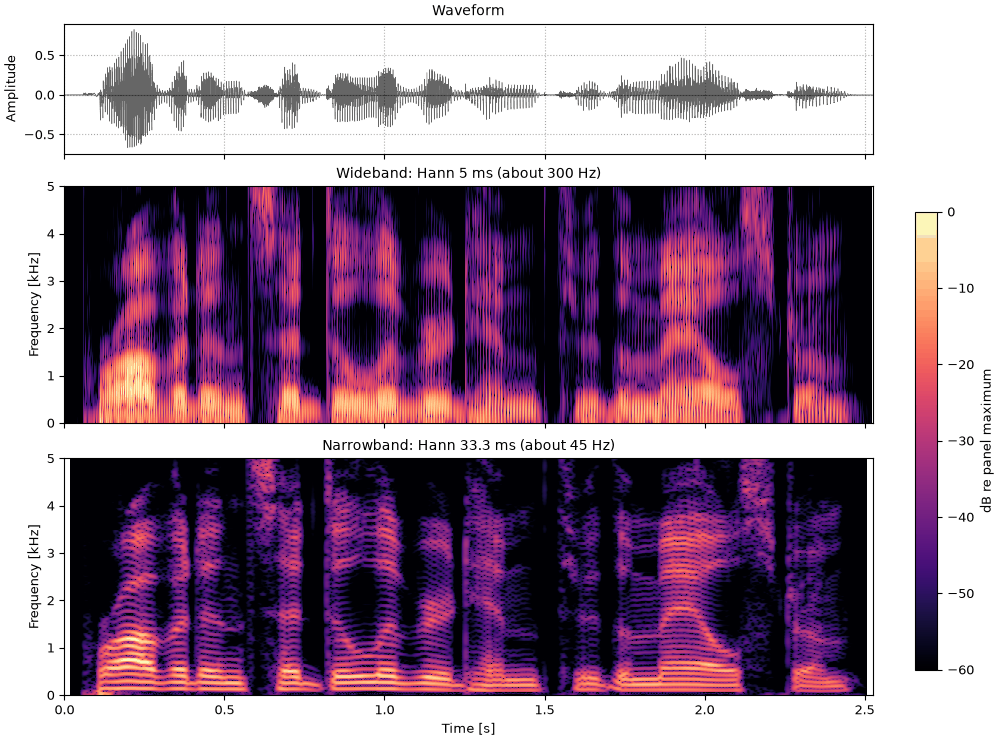
Spectrograms. One sentence through a wideband (5 ms) and a narrowband (33 ms) Gabor frame: the first resolves the glottal pulses, the second the harmonics. ▶ listen
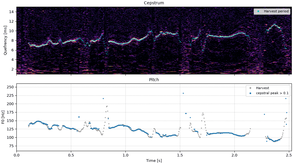
Cepstrum. The cepstrogram of the same sentence, with so.Cepstrum's F0
beside WORLD's Harvest. ▶ listen
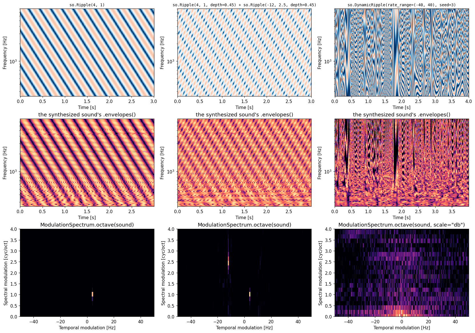
Modulation spectra. Three ripple patterns as specified (top), the
synthesized sounds' subband envelopes (middle), and their measured
so.ModulationSpectrum (bottom), which peaks at each specified rate and density.
▶ single ▶ sum of two ▶ dynamic
More in the gallery:
- Analysis and resynthesis: a filterbank's ▶ perfect reconstruction, and the ▶ ideal binary mask.
- Phase vocoder: how it works, and duration, pitch and partials changed independently, such as ▶ up a fifth.
- Spectrotemporal ripples: moving ripples on different carriers, and a ▶ dynamic moving ripple.
- Binaural cues: ▶ timing alone, and correlation that changes, such as ▶ Oscor.
- Seeing speech: a short course in time-frequency analysis on one sentence, from ▶ window length to ▶ reassignment.
- Sound textures: recordings and their syntheses from statistics (McDermott & Simoncelli, 2011), such as a ▶ stream.
- Moving talkers: three talkers rendered through measured HRIRs, ▶ one of them moving.
- Hearing through a vocoder: cochlear-implant simulation, from ▶ one band to ▶ sixteen.
- Cepstral analysis: separating a voice's pitch from its timbre, ▶ envelope only and ▶ harmonics only.
- Synthetic reverberation: rooms built from the statistics of real ones (Traer & McDermott, 2016), from a ▶ natural room to ones that break the rules, such as a ▶ time-reversed decay.
- Iterated rippled noise: a pitch made from noise and a delay (Yost, 1996), from ▶ one iteration to ▶ sixteen.
- Classic stimuli: ▶ speech-shaped noise, beats and roughness, and ▶ binaural beats.
Conventions
- Sounds.
Sound= immutable(n_samples, n_channels)float array +fs. Operations return new Sounds. - Arithmetic.
a + bmixes,a * bmultiplies sample-wise,2 * ascales, mono broadcasts to stereo. - Bands and envelopes. A filterbank's output (
Subbands) is a collection of Sounds, and so is its fine structure (.tfs()). Envelopes are not sounds:EnvelopeandEnvelopesare their own types, non-negative, often at a low sampling rate, and applied to sounds by multiplication.Envelopes(one envelope per band) is what the field calls a cochleagram. The Hilbert decomposition is literal:sb == sb.envelopes() * sb.tfs(). - Levels.
a + 6*dB,a - 3*dB. Adding a bare number is an error, so it can't be mistaken for a DC offset. dB is always20*log10(amplitude). - Time.
snd[0.1:0.5]slices by seconds;snd.datafor samples. - Randomness. Every stochastic function takes
rng=(a seed ornp.random.Generator). - Binaural. Positive ITD = right ear leads; positive ILD = right ear louder.
- Space. Meters, head-centered, x = right, y = front, z = up.
hcc= (distance cm, elevation °, azimuth ° clockwise from front). - Plots. Every plotting function takes an optional
axand returns it; global matplotlib settings are never touched.
What's in it
The modules are grouped in layers, and each imports only from the layers
listed before it here (core first); plotting is called from every
object's .plot(). docs/design/layout.md has the diagram. Most names are
also at the top level as so.name; the texture ones are under
so.texture and sonore.texture.synth.
| Module | Contents |
|---|---|
core.sound |
Sound, load |
core.units |
dB, Decibels |
signals.generators |
silence, pure_tone, harmonic_complex, schroeder_complex, square_wave, sawtooth_wave, pulse_train, linear_chirp, exponential_chirp, gaussian_noise, correlated_noise, iterated_ripple_noise |
signals.processing |
pad, truncate, concat, mix, normalize, match_fs, match_channels, relative_db, bandpass, butter_filter, amplitude_modulate |
analysis.frames |
Frame (invertible analyses: analyze, synthesize as least squares, frame_bounds, energy, adjoint), Filterbank (frequency-domain filters, any shape; canonical dual), GaborFrame (the STFT as a frame; any window, zero-padded FFTs), TVGaborFrame (a Gabor frame whose window changes over time, from an explicit schedule, from_function, or pitch_adaptive from an F0 track; exact inverse; coefficients are a TVSTFT) |
analysis.filterbank |
ERBFilterbank, OctaveFilterbank (perfect-reconstruction cosine banks sharing CosineFilterbank, a tight Filterbank), GammatoneFilterbank (exact 4th-order gammatone responses, causal or zero-phase; envelope_peak_delay gives each filter's latency), MorletFilterbank (log-spaced Morlet wavelets); both add edge filters by default so synthesis is exact on the whole band, and edges=False gives the bare bank for cochleagrams. subbands, Subbands (a collection of Sounds: .envelopes(), .tfs(), .synthesize()), noise_vocode |
analysis.representations |
Spectrum, long_term_spectrum, STFT (a GaborFrame analysis: exact inverse, fast Griffin-Lim), TVSTFT (a TVGaborFrame analysis), tandem_power (TANDEM-STRAIGHT-style pitch-adaptive power, after Kawahara et al., 2011; magnitude only, a TFPower), reassigned_spectrogram (Kodera et al., 1978; Auger & Flandrin, 1995: spectrogram cells moved to their reassigned time and frequency, binned for display; not invertible), Mask, ideal_binary_mask, ideal_ratio_mask, ModulationSpectrum (linear-frequency from an STFT, or .octave() in cycles/octave) |
analysis.cepstrum |
Cepstrum (the real cepstrum of an STFT or TVSTFT: rectangular liftering with a fixed or per-frame cutoff, the cepstral envelope, resynthesis with the original phase, exact when unliftered, or the minimum phase, and classic cepstral F0 after Noll, 1967) |
analysis.envelopes |
Envelope (one envelope; env * snd modulates), Envelopes (one per band, i.e. a cochleagram; .plot(), .modulation_spectrum(), env * subbands) |
analysis.modulation |
ConstantQModulationFilterbank, OctaveModulationFilterbank (circular, analytic output optional) |
stimuli.ripples |
Ripple, RippleSum, DynamicRipple, ripple_sound; patterns can also be any function f(t, x) of time and octaves, and pattern.render(filterbank, dur, fs) gives their Envelopes |
stimuli.phasevocoder |
time_stretch, pitch_shift (identity phase locking), pv_analyze → PVAnalysis (instantaneous frequency; oscillator-bank resynthesize with time_scale and freq_map) |
stimuli.binaural |
apply_itd_ild, simple_bir, interaural_cues, oscor, phasewarp |
stimuli.spatialization |
HRIRSet (PKU-IOA, SOFA; onset-aligned interpolation), spatialize, move_sound, trajectories, coordinate conversions, distance_gain_db |
stimuli.hrir_data |
load_hrirs: public HRIR databases (PKU-IOA) downloaded on first use, checksum-verified and cached |
stimuli.reverb |
synth_ir (natural rooms, or the paper's atypical decay_shape / rt60_profile / drr_profile variants), band_rt60s, measure_rt60 |
texture.stats |
TextureModel, TextureStats (.measure, .snr, .replace for hybrids, .save/.load) |
texture.synth |
synthesize (full loop), impose_channel; gradients in texture.grad |
plotting |
overview and the plot_* functions behind each object's .plot(); plot_tf_db draws any time-frequency level on non-uniform frames; cochleagrams take align="peak" (draw causal gammatone bands without their latency) and fscale="linear" (to match spectrograms) |
Related projects
Where to go for what sonore leaves out:
-
slab: calibrated levels in dB SPL, playback, trial sequences and adaptive staircases. Its sound making overlaps with sonore's, and the two share the same sample layout (samples × channels), so a sound passes between them in one line:
s = slab.Sound(snd.data, samplerate=snd.fs)  # sonore to slab; then set s.level in dB SPL
snd = so.Sound(s.data, s.samplerate)          # slab to sonore
slab reads samples as pascals, so a sonore sound at RMS 1 shows as 94 dB SPL until you set its level.
-
PsychoPy: running experiments.
-
Auditory Modeling Toolbox (MATLAB/Octave) and torch_amt (PyTorch): models of the auditory system that predict what a listener hears.
-
brian2hears: auditory periphery and spiking models.
-
MoSQITo: loudness, sharpness, roughness and other sound quality metrics.
-
Parselmouth (Praat in Python) and pyworld (WORLD): speech analysis and synthesis.
-
librosa: music and audio analysis.
-
pyroomacoustics: geometric room simulation.
Roadmap
Done
- Frames. A
Framecontract for invertible time-frequency analyses:analyze,synthesize(canonical dual, least-squares for modified coefficients),frame_bounds()andadjoint. The STFT (GaborFrame), the cosine, gammatone and Morlet filterbanks, and a time-varying Gabor frame with pitch-adaptive windows are all frames; tests enforcesynthesize(analyze(x)) == xand the reported bounds. Reassigned spectrograms and a TANDEM-STRAIGHT-style power spectrum are drawn beside them in the Seeing speech page. - Cepstrum.
Cepstrumon any STFT: liftering, resynthesis with the original or minimum phase, and classic cepstral F0; seedocs/design/cepstrum.md. - Package layout. One subpackage per layer (
core,signals,analysis,stimuli,texture), with imports pointing down a layer, enforced bytests/test_layers.py; seedocs/design/layout.md. - CI and releases. Tests and lint on Python 3.10 and 3.14 for every push
and pull request, a check that the PyPI files build and pass their tests,
and a trusted-publishing release workflow (
docs/releasing.md). - HRIRs on demand.
so.load_hrirs()downloads the PKU-IOA database (Qu et al., 2009) on first use, checks each file's checksum and caches it, correcting the left-right mirroring of its SOFA copy; seedocs/design/hrir-data.md. - Gallery pages. The gallery is split into pages, each a runnable script
shown with its code: Seeing speech (a short course in
time-frequency analysis), Sound textures,
Cepstral analysis (liftering, minimum phase and
cepstral F0, cross-checked against SciPy, MATLAB's
rcepsand Praat bytools/crosscheck_cepstrum.py), Hearing through a vocoder (cochlear-implant simulation withso.noise_vocode), and Moving talkers (a target talker swinging in azimuth between two still maskers, after Cho & Kidd, 2022, with interaural cues and a top-down view that follows playback). - The MSM archive. The experiment code behind Cho & Kidd (2022), written with sigtools 0.1, stays a separate archive at choyun1/MSM rather than being folded in; the Moving talkers page carries its stimuli forward.
Next, in order
- First PyPI release. The workflows are in place; what remains is publishing 0.3 to TestPyPI and then PyPI.
- JAX spike. Port the texture channel objective to JAX, check it
against the NumPy reference with the existing tests, and measure it
against today's ~2 s per iteration. On the evidence, decide on an optional
sonore[jax]backend for the heavy, optimization-shaped parts (texture synthesis now; the differentiable forward models that source inference needs later). The core stays NumPy. - Texture modulation convergence. Rebalance the objective so modulation power converges (see Texture synthesis below).
- Speech analysis and synthesis. A WORLD-style model (Morise et al., 2016; after STRAIGHT, Kawahara et al., 1999) built on the cepstrum and the pitch-adaptive frame: an F0 tracker, a CheapTrick-style spectral envelope (Morise, 2015), aperiodicity, and pulse-plus-noise synthesis. Alongside it, source-filter vowels (glottal source, formant resonators, radiation) and the Klatt synthesizer (Klatt, 1980; KLSYN88, Klatt & Klatt, 1990).
- Moving-sound renderer. Revisit
move_sound, since linear trajectories sound unconvincing: sources that change distance (level change, travel-time delay, Doppler shift and room reverberation), a sinusoidal azimuth trajectory like the one in Cho & Kidd (2022), and faster rendering via batched frequency-domain filtering. Changing-filter methods are reviewed by Brandtsegg et al. (2018); sonore's windowed switching with onset-aligned interpolation is described on the Moving talkers page.
Texture synthesis
- Rebalance the objective so modulation power converges (it reaches 30 dB SNR when imposed without the correlation classes, but 18-23 dB in full synthesis); try joint imposition of all channels.
- Impose several channels at once; the per-channel objective is overhead-bound (about 2 s per iteration for 5 s of sound).
- Validate against the MATLAB toolbox's published examples by running both on the same original recordings.
Architecture
- Model subpackages (
sonore.texture, latersonore.speech) sit on top of the layers below them and are never imported by them. Heavy dependencies go in optional extras. - Split a component into its own distribution only when it needs a heavy dependency, a different release cadence, or a separate audience.
- Bayesian inference of sound sources will be a separate package built on sonore (JAX plus a probabilistic-programming layer), using sonore's generators, frames and texture statistics as its differentiable forward model.
Other
- Free-form modulation patterns: specify a modulation spectrum and synthesize it.
- A decimated, invertible constant-Q transform (nonstationary Gabor frames in frequency).
- Peak-based sinusoidal modeling (McAulay & Quatieri, 1986) alongside the channel oscillator bank.
- On-demand download of other public HRIR databases.
References
Each entry is the citation and a link to the work: the DOI where one is confirmed, otherwise
the publisher or another stable page. After it come tags naming the module(s) in
What's in it that implement or follow the work, linked to the source: a tag such
as representations.reassigned_spectrogram goes to that definition, a bare module name to the
whole file. Last, set apart by a ·, are the gallery pages (▶) and roadmap items that cite it.
Works with no tag are not implemented yet.
- Auger & Flandrin (1995). Improving the readability of time-frequency and time-scale representations by the reassignment method. IEEE Trans. Signal Processing 43(5). doi:10.1109/78.382394.
representations.reassigned_spectrogram· ▶ Seeing speech - Balazs, Dörfler, Jaillet, Holighaus & Velasco (2011). Theory, implementation and applications of nonstationary Gabor frames. J. Comput. Appl. Math. 236(6). doi:10.1016/j.cam.2011.09.011.
frames.TVGaborFrame - Boersma & Weenink. Praat: doing phonetics by computer (computer program). praat.org. Cross-checks
Cepstrum(see Reference implementations). · ▶ Cepstral analysis - Bogert, Healy & Tukey (1963). The quefrency alanysis of time series for echoes: cepstrum, pseudo-autocovariance, cross-cepstrum and saphe cracking. In M. Rosenblatt (ed.), Time Series Analysis, Wiley. Semantic Scholar.
cepstrum.Cepstrum· ▶ Cepstral analysis - Brandtsegg, Saue & Lazzarini (2018). Live convolution with time-varying filters. Applied Sciences 8(1), 103. MDPI. Reviews the ways of filtering with a changing filter;
move_soundis one of them.spatialization.move_sound· ▶ Moving talkers · Roadmap - Byrne et al. (1994). An international comparison of long-term average speech spectra. JASA 96(4), 2108–2120. doi:10.1121/1.410152.
representations.long_term_spectrum· ▶ Classic stimuli - Chi, Gao, Guyton, Ru & Shamma (1999). Spectro-temporal modulation transfer functions and speech intelligibility. JASA 106. JASA.
ripples.Ripplerepresentations.ModulationSpectrum· ▶ Spectrotemporal ripples - Cho & Kidd (2022). Auditory motion as a cue for source segregation and selection in a "cocktail party" listening environment. JASA 152(3), 1684–1694. doi:10.1121/10.0013990. Its experiment code is archived at choyun1/MSM.
spatialization.move_soundbinaural.interaural_cues· ▶ Moving talkers · Roadmap - Christensen (2003). An Introduction to Frames and Riesz Bases. Birkhäuser. doi:10.1007/978-0-8176-8224-8.
frames.Frame - Cuevas-Rodríguez, Picinali, González-Toledo et al. (2019). 3D Tune-In Toolkit: an open-source library for real-time binaural spatialisation. PLOS ONE 14(3), e0211899. doi:10.1371/journal.pone.0211899. Removes the interaural delay before interpolating HRIRs, as sonore's onset alignment does.
spatialization.HRIRSet· ▶ Moving talkers - Daubechies, Grossmann & Meyer (1986). Painless nonorthogonal expansions. J. Math. Phys. 27(5). doi:10.1063/1.527388.
frames.GaborFrame - Dolson (1986). The phase vocoder: A tutorial. Computer Music Journal 10(4). Semantic Scholar.
phasevocoder· ▶ Phase vocoder - Dorman, Loizou & Rainey (1997). Speech intelligibility as a function of the number of channels of stimulation for signal processors using sine-wave and noise-band outputs. JASA 102(4), 2403–2411. doi:10.1121/1.420354.
filterbank.noise_vocode· ▶ Hearing through a vocoder - Escabí & Schreiner (2002). Nonlinear spectrotemporal sound analysis by neurons in the auditory midbrain. J. Neurosci. 22. doi:10.1523/JNEUROSCI.22-10-04114.2002.
ripples.DynamicRipple· ▶ Spectrotemporal ripples - Flanagan & Golden (1966). Phase vocoder. Bell System Technical Journal 45. doi:10.1002/j.1538-7305.1966.tb01706.x.
phasevocoder· ▶ Phase vocoder - Friesen, Shannon, Baskent & Wang (2001). Speech recognition in noise as a function of the number of spectral channels: comparison of acoustic hearing and cochlear implants. JASA 110(2), 1150–1163. PubMed.
filterbank.noise_vocode· ▶ Hearing through a vocoder - Gabor (1946). Theory of communication. Part 1: The analysis of information. J. IEE 93(26). doi:10.1049/ji-3-2.1946.0074.
frames.GaborFrame· ▶ Seeing speech - Gamper (2013). Head-related transfer function interpolation in azimuth, elevation, and distance. JASA 134(6), EL547. doi:10.1121/1.4828983. The HRIR interpolation used in Cho & Kidd (2022); sonore interpolates onset-aligned responses instead.
spatialization.HRIRSet.at - Glasberg & Moore (1990). Derivation of auditory filter shapes from notched-noise data. Hearing Research 47. doi:10.1016/0378-5955(90)90170-T.
filterbank.ERBFilterbank· ▶ Seeing speech ▶ Classic stimuli - Gordon & Strawn (1985). An introduction to the phase vocoder. In J. Strawn (ed.), Digital Audio Signal Processing: An Anthology. Also Stanford CCRMA report STAN-M-55. CCRMA.
phasevocoder· ▶ Phase vocoder - Griffin & Lim (1984). Signal estimation from modified short-time Fourier transform. IEEE TASSP 32. doi:10.1109/TASSP.1984.1164317.
representations.STFT.griffin_lim - Kawahara, Masuda-Katsuse & de Cheveigné (1999). Restructuring speech representations using a pitch-adaptive time-frequency smoothing and an instantaneous-frequency-based F0 extraction. Speech Communication 27. doi:10.1016/S0167-6393(98)00085-5.
frames.TVGaborFrame.pitch_adaptive· Roadmap - Kawahara et al. (2011). Technical foundations of TANDEM-STRAIGHT, a speech analysis, modification and synthesis framework. Sādhanā 36(5). doi:10.1007/s12046-011-0043-3.
representations.tandem_power· ▶ Seeing speech - Klatt (1980). Software for a cascade/parallel formant synthesizer. JASA 67(3). doi:10.1121/1.383940. · Roadmap
- Klatt & Klatt (1990). Analysis, synthesis, and perception of voice quality variations among female and male talkers. JASA 87. doi:10.1121/1.398894. · Roadmap
- Kodera, Gendrin & de Villedary (1978). Analysis of time-varying signals with small BT values. IEEE Trans. ASSP 26(1). doi:10.1109/TASSP.1978.1163047.
representations.reassigned_spectrogram· ▶ Seeing speech - Kominek & Black (2004). The CMU Arctic speech databases. Proc. 5th ISCA Speech Synthesis Workshop (SSW5), 223–224. ISCA Archive. The gallery's speech (speakers bdl and rms; see
docs/speech/SOURCES.md). · ▶ Seeing speech ▶ Cepstral analysis ▶ Hearing through a vocoder ▶ Moving talkers ▶ Synthetic reverberation ▶ Phase vocoder ▶ Classic stimuli - Kowalski, Depireux & Shamma (1996). Analysis of dynamic spectra in ferret primary auditory cortex. I. J. Neurophysiol. 76. doi:10.1152/jn.1996.76.5.3503.
ripples.Ripple· ▶ Spectrotemporal ripples - Laroche & Dolson (1999). Improved phase vocoder time-scale modification of audio. IEEE Trans. Speech Audio Process. 7(3). IEEE Xplore.
phasevocoder.time_stretch· ▶ Phase vocoder - Licklider, Webster & Hedlun (1950). On the frequency limits of binaural beats. JASA 22(4), 468–473. doi:10.1121/1.1906629. · ▶ Classic stimuli
- McAulay & Quatieri (1986). Speech analysis/synthesis based on a sinusoidal representation. IEEE TASSP 34. Internet Archive. · Roadmap
- McDermott & Simoncelli (2011). Sound texture perception via statistics of the auditory periphery. Neuron 71. doi:10.1016/j.neuron.2011.06.032.
texturefilterbank.CosineFilterbankmodulation· ▶ Sound textures ▶ Analysis and resynthesis - Morise (2015). CheapTrick, a spectral envelope estimator for high-quality speech synthesis. Speech Communication 67. doi:10.1016/j.specom.2014.09.003.
frames.TVGaborFrame.pitch_adaptive· ▶ Cepstral analysis · Roadmap - Morise, Yokomori & Ozawa (2016). WORLD: A vocoder-based high-quality speech synthesis system for real-time applications. IEICE Trans. Inf. & Syst. E99-D(7). doi:10.1587/transinf.2015EDP7457. · ▶ Seeing speech ▶ Cepstral analysis · Roadmap
- Noll (1967). Cepstrum pitch determination. JASA 41(2). PubMed.
cepstrum.Cepstrum.f0· ▶ Cepstral analysis - Oppenheim & Schafer (2010). Discrete-Time Signal Processing, 3rd ed., ch. 13. Pearson. Pearson.
cepstrum.Cepstrum.to_stft· ▶ Cepstral analysis - Patterson, Robinson, Holdsworth, McKeown, Zhang & Allerhand (1992). Complex sounds and auditory images. In Auditory Physiology and Perception (Proc. 9th International Symposium on Hearing). doi:10.1016/B978-0-08-041847-6.50054-X.
filterbank.GammatoneFilterbank - Perraudin, Balazs & Søndergaard (2013). A fast Griffin-Lim algorithm. IEEE WASPAA. doi:10.1109/WASPAA.2013.6701851.
representations.STFT.griffin_lim - Plomp & Levelt (1965). Tonal consonance and critical bandwidth. JASA 38(4), 548–560. doi:10.1121/1.1909741. · ▶ Classic stimuli
- Qu et al. (2009). Distance-dependent head-related transfer functions measured with high spatial resolution using a spark gap. IEEE TASLP 17. PKU Scholar.
spatialization.HRIRSet.from_pku_ioahrir_data.load_hrirs· ▶ Moving talkers - Schroeder (1970). Synthesis of low-peak-factor signals and binary sequences with low autocorrelation. IEEE Trans. Inf. Theory 16. doi:10.1109/TIT.1970.1054411.
generators.schroeder_complex - Shannon et al. (1995). Speech recognition with primarily temporal cues. Science 270. doi:10.1126/science.270.5234.303.
filterbank.noise_vocode· ▶ Hearing through a vocoder - Singh & Theunissen (2003). Modulation spectra of natural sounds and ethological theories of auditory processing. JASA 114(6). doi:10.1121/1.1624067.
representations.ModulationSpectrumenvelopes.Envelopes.modulation_spectrum· ▶ Spectrotemporal ripples - Siveke et al. (2008). Psychophysical and physiological evidence for fast binaural processing. J. Neurosci. 28. J. Neurosci..
binaural.oscorbinaural.phasewarp· ▶ Binaural cues - Traer & McDermott (2016). Statistics of natural reverberation enable perceptual separation of sound and space. PNAS 113. doi:10.1073/pnas.1612524113.
reverb.synth_ir· ▶ Synthetic reverberation - Wang (2005). On ideal binary mask as the computational goal of auditory scene analysis. In Speech Separation by Humans and Machines. doi:10.1007/0-387-22794-6_12.
representations.ideal_binary_mask· ▶ Analysis and resynthesis - Wilson, Finley, Lawson, Wolford, Eddington & Rabinowitz (1991). Better speech recognition with cochlear implants. Nature 352, 236–238. PubMed.
filterbank.noise_vocode· ▶ Hearing through a vocoder - Yost (1996). Pitch of iterated rippled noise. JASA 100. JASA (PDF).
generators.iterated_ripple_noise· ▶ Iterated rippled noise
Reference implementations
Implementations by a paper's authors or widely used ports, with how sonore
relates to each. "Cross-checked" means a script in tools/ compares the two
numerically; "consulted" means the code was read for behavior but not copied.
- Sound Texture Synthesis Toolbox v1.7 (MATLAB), McDermott lab: the
authors' implementation of McDermott & Simoncelli (2011). Consulted; sonore
is a clean-room implementation from the paper, and every deliberate
difference is listed in
so.texture.DIFFERENCES_FROM_TOOLBOX.texturefilterbank.CosineFilterbankmodulation - wil-j-wil/texture_stats (Python, MIT): a port of the toolbox's
statistics. Cross-checked by
tools/crosscheck_texture_stats.py.texture.TextureStats - mcdermottLab/pycochleagram (Python): the lab's port of the
toolbox's cochleagram code, including the cosine filterbank. Not yet
cross-checked.
filterbank.CosineFilterbank - LTFAT (MATLAB/Octave, GPLv3):
frsynabswith'fgriflim'is the fast Griffin-Lim from the group of Perraudin, Balazs & Søndergaard (2013);librosa.griffinlimis a widely used Python version. Neither is cross-checked yet.representations.STFT.griffin_lim - SciPy
ShortTimeFFT(BSD-3): wrapped byGaborFrame. Its frame operator, bounds and least-squares inverse are cross-checked against dense matrices in the tests and intools/check_frames_step1_claims.py(docs/design/frames.md, step 1).frames.GaborFramerepresentations.STFT - Gammatone filterbanks in Slaney's Auditory Toolbox and MATLAB's
gammatoneFilterBankare time-domain IIR approximations;GammatoneFilterbankuses the exact frequency response instead (derivation in docs/design/frames.md, step 2). Consulted for conventions only.filterbank.GammatoneFilterbank - SciPy
minimum_phase(homomorphic method), the real-cepstrum definition MATLAB'srcepsdocuments, and Praat's PowerCepstrogram through parselmouth (GPLv3): cross-checked bytools/crosscheck_cepstrum.py, Praat at development time only.cepstrum.Cepstrum - LTFAT (GPLv3) and nsgt (Artistic License 2.0):
frame theory in code, for dev-time cross-checks only because of their licenses. Not yet cross-checked.
frames
Migrating from sigtools
sonore was previously sigtools, renamed to avoid a clash with an unrelated
PyPI package of that name. Version 0.2 also redesigned the API:
| sigtools 0.1 | sonore |
|---|---|
from sigtools.sounds import * etc. |
import sonore as so |
PureTone(dur, fs, f), GaussianNoise(...), ... |
so.pure_tone(dur, fs, f), so.gaussian_noise(...), ... |
GaussianNoise(dur, fs, lo, hi, tilt) |
so.gaussian_noise(dur, fs, band=(lo, hi), tilt=...); tilt is now dB/octave |
SchroederPhase(dur, fs, f0, n) |
so.schroeder_complex(dur, fs, f0, n) |
SoundLoader(path), Silence(dur, fs) |
so.load(path), so.silence(dur, fs) |
snd + 6 (dB gain) |
snd + 6*dB |
snd.make_binaural(), snd.extract_envelope() |
snd.to_stereo(), snd.envelope() (now returns an Envelope, not a Sound) |
ramp_edges(snd, d) |
snd.ramp(d) |
butter_bandpass_filter(snd, lo, hi) |
so.bandpass(snd, lo, hi) (no longer RMS-normalizes) |
equalize_fs, zeropad_sounds, center_sounds, truncate_sounds |
so.match_fs, so.pad(align="start"/"center"), so.truncate |
normalize_rms, zero_mean, concat_sounds, compare_relative_db |
so.normalize, snd.zero_mean(), so.concat, so.relative_db |
sum(zeropad_sounds([a, b])) |
so.mix([a, b]) |
MagnitudeSpectrum(s).to_Noise(dur, fs) |
so.long_term_spectrum(s).to_noise(dur, fs) |
STFT(snd, win), S.to_Sound(), method="GLA" |
so.STFT(snd, win), S.to_sound(), S.griffin_lim() |
IBM = S_t > S_m + lc; IBM * S_mix |
so.ideal_binary_mask(S_t, S_m, lc_db=lc); S_mix * mask |
Subbands(snd, n), .extract_envelopes(), .to_Sound() |
so.subbands(snd, n), .envelopes(), .synthesize() |
InterauralCues(snd, win) |
so.interaural_cues(snd, win) |
SimpleBIR(fs, itd, ild) |
so.simple_bir(fs, itd, ild) or so.apply_itd_ild(snd, itd, ild) |
SynthIR(drr, rt60, dB_thresh, fs) |
so.synth_ir(rt60, fs, drr_db=..., decay_db=-dB_thresh) |
move_sound(traj, snd) |
so.move_sound(snd, traj, hrirs) with so.load_hrirs() (downloads PKU-IOA), so.HRIRSet.from_pku_ioa(dir) or .from_sofa(path) |
display_STFT(x, S), AudioControl(snd).display() |
so.overview(x); put snd at the end of a cell |
Results computed with 0.1 can differ, because these 0.1 bugs were fixed:
spectrum and STFT "dB" were half the true value; the bandpass filter filtered
stereo across channels; SimpleBIR was a sample short and got louder with
larger ITDs; SynthIR's DRR had no effect and its resynthesis filters were
shifted in frequency; tone frequencies were off by a factor of (n-1)/n;
move_sound summed ~100 unwindowed overlapping convolutions per sample; and IAC
was never computed. The ILD in apply_itd_ild is now split ±ILD/2 across the
ears (0.1 applied it to the right ear only).
Development
pip install -e ".[dev]"
pytest                             # ~40 s; one test file per module
ruff check . && ruff format .
python docs/gallery/build.py       # regenerate the listening gallery (a few minutes)
How sonore was developed
sonore began as sigtools, the code I (Adrian Cho) wrote in graduate school to make psychoacoustic stimuli. The 0.2 redesign and everything since were developed together with Claude, Anthropic's AI assistant, in chat sessions during 2026.
What Claude did. Wrote most of the code, tests, documentation, and gallery since 0.2, delivered as patches; drafted design documents; ran numerical checks and profiling; and looked up and checked citations.
What I did. Decided what sonore is for and what goes in it, including its API conventions, the texture work and its milestones, and the roadmap and architecture. I chose and documented the texture recordings and set the working rules: implement from the papers, verify every claim numerically, document every deviation and data choice, and write a design document before large features. I reviewed and applied each patch. The design principles that came out of this are summarized in docs/design/philosophy.md.
How it is verified. I have not read every line by hand. What I rely on instead is the following:
- The test suite, with one file per module.
- Finite-difference and dense-matrix checks of the mathematics.
- Cross-checks against independent implementations (see "Reference implementations").
- Written records of every decision (
DIFFERENCES_FROM_TOOLBOX,docs/textures/SOURCES.md,docs/design/). - The listening gallery, since these are sounds and should be heard.
I am responsible for sonore's correctness. If something is wrong, please open an issue.
License and citation
MIT; see LICENSE. If sonore is useful in your research, please cite it using CITATION.cff.
1 maintainer

Metadata
1 maintainer
Release files for sonore 0.3.0
For a detailed explanation of source distributions (sdists) and built distributions (wheels), please see the package formats documentation.
Source distribution (sdist)
| File | Size | Uploaded | |
|---|---|---|---|
| sonore-0.3.0.tar.gz | 170.8 kB | Details |
Built distribution (wheel)
| File | Interpreter | ABI | Platform | Reset |
|---|---|---|---|---|
| sonore-0.3.0-py3-none-any.whl | Python 3 | none | any | Details |
Total release size: 284.8 kB
Release files / sonore-0.3.0.tar.gz
| Download URL | sonore-0.3.0.tar.gz |
|---|---|
| Size | 170.8 kB |
| Tags | Source |
|
SHA-256 checksum How to use checksums |
d8a8e9c37ab401aa063f612c841c3c4ffea9bd141f6e6eac34cc99cdda4c6133
|
|
BLAKE2b-256 checksum How to use checksums |
4e518ac5c21e46932744f39148669a6cfc12da551e4c7d25f3368a9d0b322d9d
|
| Upload date | |
|
Uploaded using Trusted Publishing? What is trusted publishing? |
Yes |
| Uploaded via |
twine/7.0.0 CPython/3.13.14
|
Provenance
Provenance describes where a file came from. On PyPI, provenance is shared via attestations, which provide a verifiable record of the build or publishing details. View details, limitations and caveats.


PyPI Publish Attestation
PyPI verified that this artifact, at this checksum, originated from the publisher listed below.
Signed by GitHub Actions, verified by PyPI on Oct 1, 2026.
Transparency logRelease files / sonore-0.3.0-py3-none-any.whl
| Download URL | sonore-0.3.0-py3-none-any.whl |
|---|---|
| Size | 113.9 kB |
| Tags | Python 3 |
|
SHA-256 checksum How to use checksums |
e091f653f0dd239168f8420976010091c235ae14c3fb94c7ccbc7ccb66bfa444
|
|
BLAKE2b-256 checksum How to use checksums |
08accac3d2fb8df63becd9bf97b71d709a381818ec68807df5d5f66f8bec4627
|
| Upload date | |
|
Uploaded using Trusted Publishing? What is trusted publishing? |
Yes |
| Uploaded via |
twine/7.0.0 CPython/3.13.14
|
Provenance
Provenance describes where a file came from. On PyPI, provenance is shared via attestations, which provide a verifiable record of the build or publishing details. View details, limitations and caveats.
PyPI Publish Attestation
PyPI verified that this artifact, at this checksum, originated from the publisher listed below.
Signed by GitHub Actions, verified by PyPI on Oct 1, 2026.
Transparency log













