Given a FITS spectrum file, this script fits a Voigt profile to each emission line, facilitating flux calculation and data validity assessment. It generates plots for each line and outputs comprehensive results in both FITS and ECSV formats. These files contain all necessary information for analysis or reproduction.

Project description
spec2flux
About spec2flux
Spec2flux (Spectrum to Flux) aims to accurately calculate the emission line flux of lines in the Far Ultraviolet (FUV) range. This range contains information that can help clue in on exoplanetary atmospheres with the measurements providing insight into FUV radiation from host stars. Integrating UV spectra with X-ray data allows us to estimate the stellar corona, adding to the toolkit of exoplanet atmosphere data.
How it works
The script accomplishes the task of calculating flux by:
- Grouping emission lines using a preset tolerance, which can be adjusted if using a different DEM file.
- Calculating the Doppler shift by fitting a composite Voigt profile to the strongest emission lines, and comparing Voigt peaks to rest wavelength to calculate.
- Iterating through each line, determining if noise, and then calculating the flux either using the Voigt profile or the original data.
- Presents a final plot of all of the final emission lines, and exports the calculations as a FITS and ECSV file.
Prerequisites


Pip Installation
-
Pip install the repository in your desired directory.
pip install spec2flux
-
Create a
main.py, which will used to put the package attributes. -
Ensure your files for the DEM lines, airglow, and the spectrum which will used to calculate the flux are in your directory.
   project-directory/
   ├── main.py
   ├── DEM_goodlinelist.csv
   ├── airglow.csv
   ├── spectrum.fits
-
Make your
main.pyresemble the following:import spec2flux def main(): # Spectrum details (adjust me with each star) spectrum_dir = 'spectrum-spec.fits' rest_dir = 'DEM_goodlinelist.csv' airglow_dir = 'airglow.csv' observation = 'sci' # SCI only telescope = 'hst' # HST only instrument = 'stis' # STIS or COS only grating = 'e140m' # L or M grating only star_name = 'NEWEX' min_wavelength = 1160 # Spectrum adjustments apply_smoothing = False # True if want to apply gaussian smoothing line_fit_model = 'Voigt' # 'Voigt' or 'Gaussian' fit # User adjustable parameters fresh_start = True # True if first time running, or have already ran for a star and want to see final plot # Check inputs spec2flux.InputCheck(spectrum_dir, rest_dir, airglow_dir, observation, telescope, instrument, grating, star_name, min_wavelength, apply_smoothing, line_fit_model, fresh_start) # Load spectrum data and emission lines spectrum = spec2flux.SpectrumData(spectrum_dir, rest_dir, airglow_dir, observation, telescope, instrument, grating, star_name, min_wavelength, apply_smoothing) emission_lines = spec2flux.EmissionLines(spectrum) # Calculate flux flux_calc = spec2flux.FluxCalculator(spectrum, emission_lines, fresh_start, line_fit_model) # Show final plot spectrum.final_spectrum_plot(emission_lines, flux_calc) if __name__ == '__main__': main()
-
Run
main.py.python main.py
-
Select "best" doppler shift candidates.
A series of plots will appear, click 'y' if the plot is an eligible candidate for doppler shift, 'n' if it is not.Figure 1: This is a good example because the Doppler shift is consistent between both emission lines, with minimal noise.
-
After iterating through all the doppler shift candidates, plots will appear for the noise selection portion.
To select if the current plot is noise or not, click 'y' if the plot is noise and 'n' if the plot is not noise.Figure 2: This plot is not noisy because the emission lines are well-defined at the specified rest wavelengths.
Figure 3: This plot is noisy because the emission lines at the specified rest wavelength are not well-defined.
-
After all emission lines are iterated through, a final plot will appear
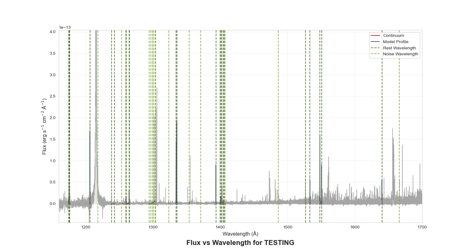
Figure 4: Plot of the entire spectrum with the continuum, profile fits, and wavelengths marked.
Figure 5: Final plot zoomed in.
-
After running the script, your directory will now look like the following:
project-directory/
├── main.py
├── DEM_goodlinelist.csv
├── airglow.csv
├── spectrum.fits
├── doppler/
│   ├── newex_doppler.txt
├── emission_lines/
│   ├── newex_lines.json
├── flux/
│   ├── newex.csv
    ├── newex.ecsv
    ├── newex.fits
├── plots/
│   ├── newex_final_plot.png


Using the data:
Header contains:
- DATE: date flux was calculated
- FILENAME: name of the fits file used to for flux calc
- TELESCP: telescope used to measure spectrum
- INSTRMNT: active instrument to measure spectrum
- GRATING: grating used to measure spectrum
- TARGNAME: name of star used in measurement
- DOPPLER: doppler shift used to measure flux
- WIDTH: average peak width of the emissoin lines
- RANGE: flux range used to isolate emission line
- WIDTHPXL: average emission line peak width in pixels
- UPPRLIMIT: upper limit used for noise
ECSV + CSV Data: File columns are Ion, Rest Wavelength, Flux, Error, Blended Line, each row representing a grouped emission line.
FITS Data: FITS Table contains the same data as the ECSV file.
Note: Noise is marked as having the negative of the upper limit (3*error) as the flux and an error of 0.


Download files
Download the file for your platform. If you're not sure which to choose, learn more about installing packages.
Source Distribution
Built Distribution
Filter files by name, interpreter, ABI, and platform.
If you're not sure about the file name format, learn more about wheel file names.
Copy a direct link to the current filters
File details
Details for the file spec2flux-0.1.3.tar.gz.
File metadata
- Download URL: spec2flux-0.1.3.tar.gz
- Upload date:
- Size: 16.9 kB
- Tags: Source
- Uploaded using Trusted Publishing? No
- Uploaded via: twine/5.1.1 CPython/3.12.5
File hashes
| Algorithm | Hash digest | |
|---|---|---|
| SHA256 |
90d6413e2c62a5b4f27ba809bfc83df13b2bac6ffd67ff7bb476ea6c46499e79
|
|
| MD5 |
73336caeae86fe916012351a61bfedcd
|
|
| BLAKE2b-256 |
f50c2cf9894990f0a5c699c39dd94ab1bba1927d2a263e80988a48c6a02801e5
|
File details
Details for the file spec2flux-0.1.3-py3-none-any.whl.
File metadata
- Download URL: spec2flux-0.1.3-py3-none-any.whl
- Upload date:
- Size: 16.0 kB
- Tags: Python 3
- Uploaded using Trusted Publishing? No
- Uploaded via: twine/5.1.1 CPython/3.12.5
File hashes
| Algorithm | Hash digest | |
|---|---|---|
| SHA256 |
58677b22eb1fcf85df91dbab0e0345e492cc4b9187c83bab71e421f0bedcfcc2
|
|
| MD5 |
5d7ab26b6c4c526329c7a21860fabb3e
|
|
| BLAKE2b-256 |
40d15a77f601a9caabf17b848c0b6bf322b3d17eee01a1a2fb4710402079c6d4
|


