
Squeeze Kernel Covariance Estimator




A streaming covariance estimator for panels of financial returns whose entire public surface is one number — the decay lam of the anchor correlation timescale. Every other quantity is derived from it, fixed by a structural argument, or computed online from the estimator's own state. An O(Kn²) state update per day, positive semi-definite by construction, missing values handled natively, no tuning, no refits. Only dependency: NumPy.
from squeeze_kernel import SqueezeKernel

sk = SqueezeKernel(lam=0.996)        # the entire public surface
for r_t in returns:                  # NaN marks missing assets
    sk.update(r_t)
cov = sk.covariance()
Reference: "The Squeeze Kernel Covariance Estimator: Dual-Timescale Tracking with Adaptive Shrinkage" (Kende, 2026) — SSRN abstract 6455918; the 2.0 estimator is described in the paper's current revision.
Why
Markets do not keep calendar time. Following Mandelbrot, the estimator treats a panel as a collection of partially coupled markets, each advancing on its own activity-driven clock — and reads those clocks from the panel's own correlation structure, so a hot cluster (say precious metals and FX) advances its correlation state while an idle one (agriculture) does not, without anyone identifying a cluster. On those clocks it runs a single recursion that:
- is PSD at every step, structurally — the correlation state evolves by a diagonal-congruence flow (a congruence plus a rank-one term); no eigenvalue clipping, no nearest-PSD repair, and no factorisation anywhere in the state update. (The adaptive timescale weights are the one exception: they read each timescale's predictive likelihood, which costs one Cholesky per timescale per day. Turn them off and the estimator is pure
O(Kn²).) - learns in market time and forgets in calendar time — observations enter with a saturating, self-studentising weight (no day counts more than one unit of trading time); memory decays at fixed per-day rates on a geometric ladder of three timescales
(lam⁴, lam, lam^¼). Pairs accrue covariance at the geometric mean of their two clock increments, which is the most positive semi-definiteness allows and exactly the Cauchy–Schwarz bound on how far two assets' clocks can overlap; - regularises itself — each timescale's shrinkage intensity is computed from two online statistics, the concentration
n/ν(dimension per unit trading time) and the de-noised fraction of correlation dispersion the target explains; the target is the Hadamard square of the running correlation, which is exactly the correlation matrix of the squared returns (cluster-respecting, PSD by the Schur product theorem, and sign-blind by construction — the signs are carried by the unshrunk term); - adapts its memory to regime breaks, in both stages — the timescale mix moves by an exponentiated-gradient step on the blend's own log score (not on any single timescale's, which would select rather than blend), at a temperature calibrated so that uninformative evidence leaves the mix within a factor e of its prior; the marginal variance is tracked on its own three-rung ladder, two octaves below the correlation ladder, and pooled panel-wide by the same rule on saturated evidence, so one spike day cannot hand a stale rung weeks of weight. Nothing in either mixture is fitted: the ladders are derived from
lam, the evidence memory is the fastest rung's, and the temperature is the null's; - ingests missing values natively — listings, delistings, halts enter as
NaN; - is fast — one Cholesky and one triangular solve per day; a thirty-year daily pass at n=300 runs in about two minutes single-threaded, well under daily rolling-window refits.
Evidence. On thirty years of S&P 500 constituents against an eleven-method field (EWMA, DCC, Ledoit–Wolf, OAS, nonlinear shrinkage, RMT filtering, Gerber, IEWMA, CM-IEWMA, and the published v1 estimator) it leads at every universe size from 50 to 300 and is the sole member of the 90% model confidence set at every size. Carried zero-shot to a diversified panel of 121 futures across eight asset classes it beats the same field calibrated on that panel's own history — matched-backbone IEWMA by 6.9 NLL/day (p = 4·10⁻⁴), calibrated DCC by 17.9 — out-of-time.
See the difference
A passive strategy any allocator would recognize: long-only minimum-variance over 300 liquid US stocks, scaled to a 15% volatility target, rebalanced monthly, 5 bps costs. Two runs on identical data; the only difference is the covariance matrix. The Squeeze Kernel arm runs SqueezeKernel(lam=0.996) — nothing tuned on this panel.
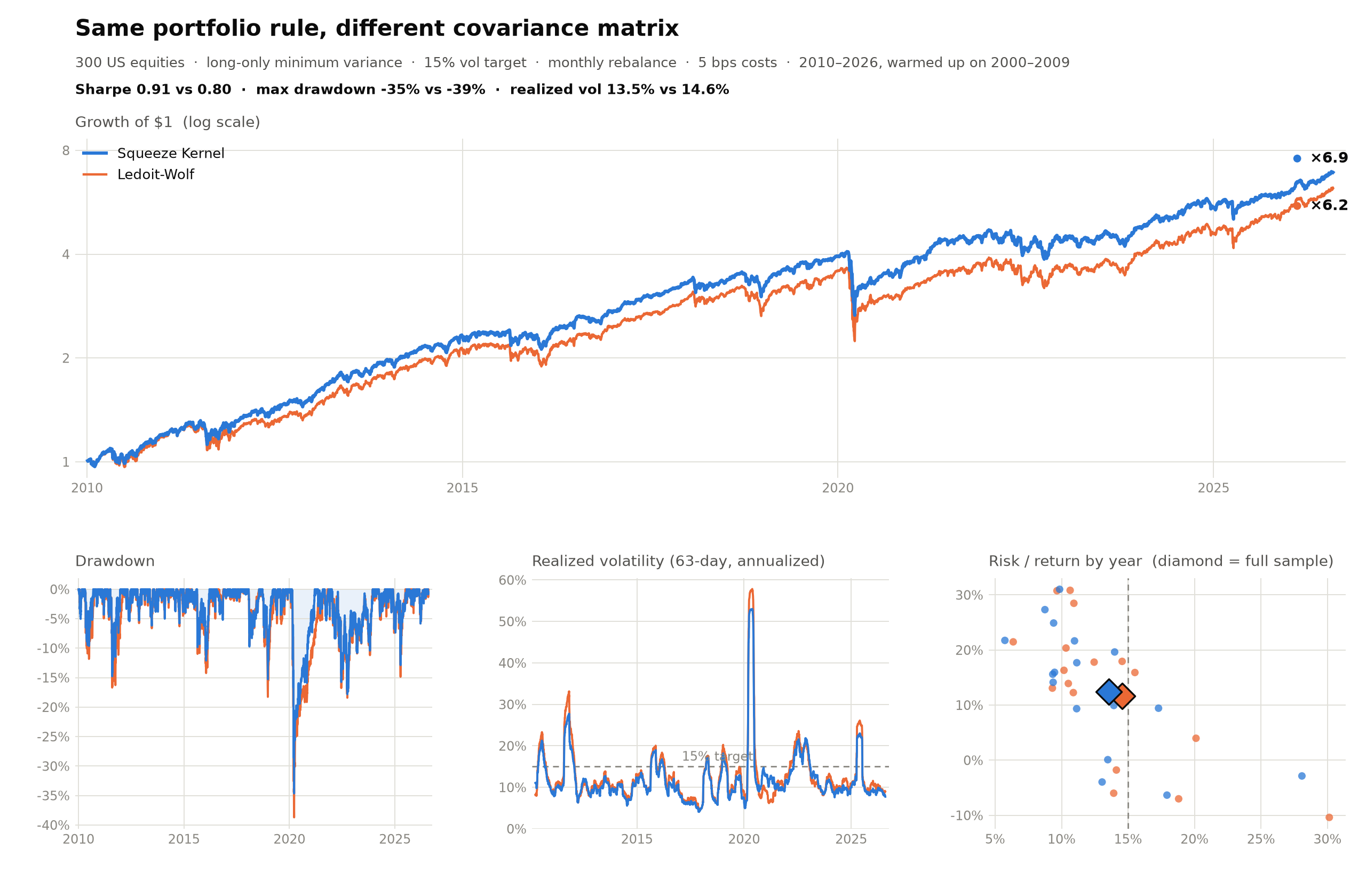
| Method | CAGR | Vol | Sharpe | MaxDD | Calmar | Vol-target RMSE |
|---|---|---|---|---|---|---|
| Squeeze Kernel (default) | 12.4% | 13.5% | 0.91 | -34.6% | 0.36 | 7.10% |
| Ledoit-Wolf (252d) | 11.7% | 14.6% | 0.80 | -38.7% | 0.30 | 7.51% |
Reproduce from the repo alone (the 300-stock panel ships as a parquet; survivorship and provenance are documented in the script):
pip install squeeze-kernel pandas pyarrow scikit-learn matplotlib
python examples/vol_targeted_portfolio.py    # ~2 minutes
Installation
pip install squeeze-kernel          # NumPy only
pip install "squeeze-kernel[full]"  # + SciPy (faster detector factorisations)
Quickstart
import numpy as np
from squeeze_kernel import SqueezeKernel, estimate_squeeze_cov

returns = np.random.default_rng(42).normal(0.0, 0.01, size=(500, 30))

sk = SqueezeKernel()                 # lam=0.996 (anchor half-life ~173 days)
for r_t in returns:
    w = sk.update(r_t)               # returns the day's kernel weight
cov, corr = sk.covariance(), sk.correlation()
sk.state()                           # kernel scale, per-timescale effective sizes, mixture tilt

# batch mode: full panel in, covariance path out
cov_path, corr_path, weights = estimate_squeeze_cov(returns, with_weights=True)
Missing values: pass NaN (or mask= on update). Newly listed, delisted or halted assets need no imputation and no complete-case subsetting.
What derives from lam
| quantity | value |
|---|---|
| timescale ladder | decays (lam⁴, lam, lam^¼) — half-lives (h/4, h, 4h), h = -1/log2(lam) |
| kernel scale | state: κ_t = ⅓ · EWMA(activity) at the anchor rate |
| shrinkage intensity | per timescale, α = min(1,c) · g̃²/(g̃² + (1−g̃)²·max(0, 1/c − 1)) from the online concentration c = n/ν and target-fit g̃ |
| timescale weights | prior ∝ √h, moved by exponentiated gradient on the blend log score at the null temperature, fast-rung memory |
| volatility memory | ladder (h/16, h/4, h), pooled panel-wide by the same rule on tanh-saturated evidence, uniform prior |
| structural constants | K=3, b=4, θ=½, κ-scale ⅓, Schur power 2 — each bracketed by ablation in the paper |
| fitted constants | none (the 2.x volatility clock λ_v = 0.98 is replaced by the ladder above) |
from squeeze_kernel import CONSTANTS exposes the structural constants for research. The published v1 estimator (all its knobs) remains available as SqueezeKernelEstimator / SqueezeKernel.v1(...); every 2.0 mechanism is also an estimator-level switch for ablation. See MIGRATION.md.
How it works
One daily update: variance on a three-rung ladder per asset, pooled by panel-wide self-adapting weights → standardised surprise → per-asset clock increments from the Schur-square-weighted neighbourhood mean of squared surprises → diagonal-congruence update of each timescale's correlation state on those clocks → per-timescale shrinkage as a learned pool of the raw correlation, its equicorrelation level and its Hadamard square, with the self-tuning intensity rule as the prior and the blend gradient as the correction → blend across timescales, moved by the gradient of the blend's own log score → covariance. The paper gives the derivations, guarantees (PSD, conditioning floor, exact reductions to the published special cases), and the full evaluation.
Development
uv sync --extra full --extra dev
uv run python -m pytest        # test suite
uv run python -m ruff check .  # lint
uv run mypy                      # strict type check (src/squeeze_kernel)
uv build                       # build sdist + wheel
Citation
@article{kende2026squeeze,
  title  = {The Squeeze Kernel Covariance Estimator: Dual-Timescale Tracking with Adaptive Shrinkage},
  author = {Kende, Robert},
  year   = {2026},
  note   = {Available at SSRN: \url{https://ssrn.com/abstract=6455918}}
}
See also CITATION.cff.
License
MIT
1 maintainer

Release files for squeeze-kernel 3.1.0
For a detailed explanation of source distributions (sdists) and built distributions (wheels), please see the package formats documentation.
Source distribution (sdist)
| File | Size | Uploaded | |
|---|---|---|---|
| squeeze_kernel-3.1.0.tar.gz | 22.3 kB | Details |
Built distribution (wheel)
| File | Interpreter | ABI | Platform | Reset |
|---|---|---|---|---|
| squeeze_kernel-3.1.0-py3-none-any.whl | Python 3 | none | any | Details |
Total release size: 47.5 kB
Release files / squeeze_kernel-3.1.0.tar.gz
| Download URL | squeeze_kernel-3.1.0.tar.gz |
|---|---|
| Size | 22.3 kB |
| Tags | Source |
|
SHA-256 checksum How to use checksums |
922db9081a99f061b88f65bf4fe8c2f555007f4f8738eebfc9edf19c8255e554
|
|
BLAKE2b-256 checksum How to use checksums |
79e3f291842b7decb2471f7d075222a47c81d83d5ae4cfb64411cc42048450f8
|
| Upload date | |
|
Uploaded using Trusted Publishing? What is trusted publishing? |
Yes |
| Uploaded via |
twine/7.0.0 CPython/3.13.14
|
Provenance
Provenance describes where a file came from. On PyPI, provenance is shared via attestations, which provide a verifiable record of the build or publishing details. View details, limitations and caveats.


PyPI Publish Attestation
PyPI verified that this artifact, at this checksum, originated from the publisher listed below.
Signed by GitHub Actions, verified by PyPI on Sep 19, 2026.
Transparency logRelease files / squeeze_kernel-3.1.0-py3-none-any.whl
| Download URL | squeeze_kernel-3.1.0-py3-none-any.whl |
|---|---|
| Size | 25.2 kB |
| Tags | Python 3 |
|
SHA-256 checksum How to use checksums |
28a372ea2f31a033f95b9b67e8b9a761f6401307e4f704654726c84aa126f290
|
|
BLAKE2b-256 checksum How to use checksums |
fe6b6c02ec283dc59df0a290ff847e89acfe1b32443d93677142fceea7149f54
|
| Upload date | |
|
Uploaded using Trusted Publishing? What is trusted publishing? |
Yes |
| Uploaded via |
twine/7.0.0 CPython/3.13.14
|
Provenance
Provenance describes where a file came from. On PyPI, provenance is shared via attestations, which provide a verifiable record of the build or publishing details. View details, limitations and caveats.
PyPI Publish Attestation
PyPI verified that this artifact, at this checksum, originated from the publisher listed below.
Signed by GitHub Actions, verified by PyPI on Sep 19, 2026.
Transparency log













