
subwave
Data-driven decomposition of neurophysiological event waveform populations.
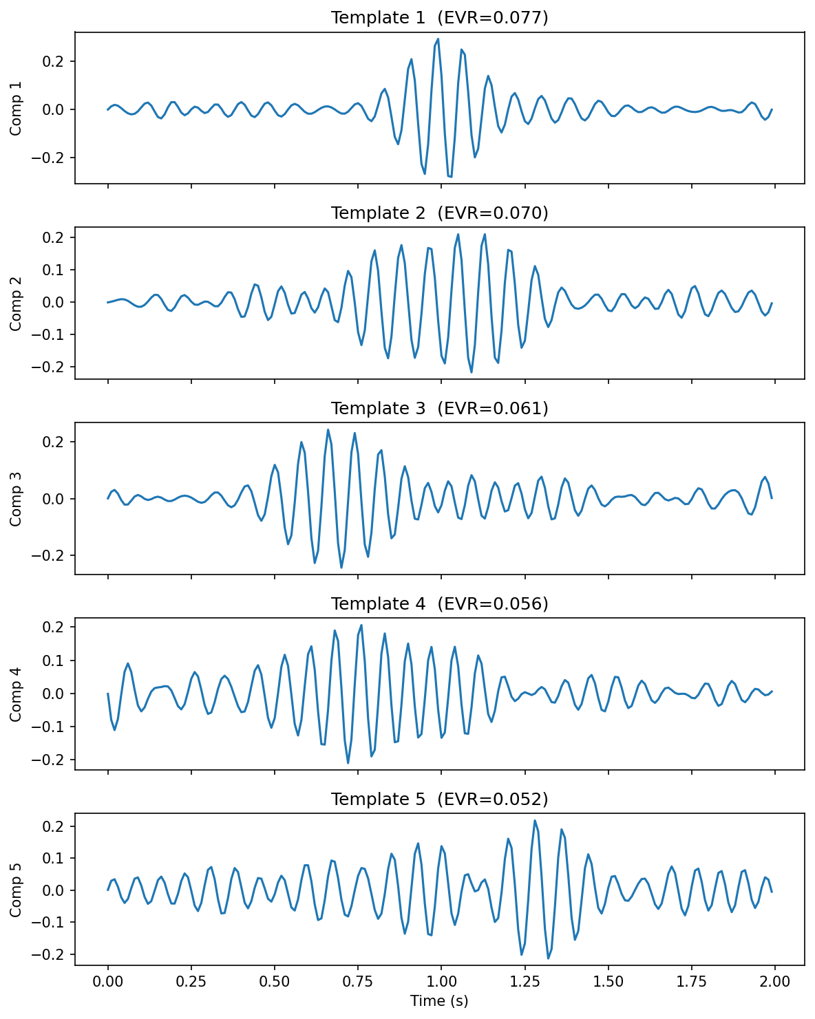
Five principal waveform templates extracted from 821 sleep spindles via SVD.
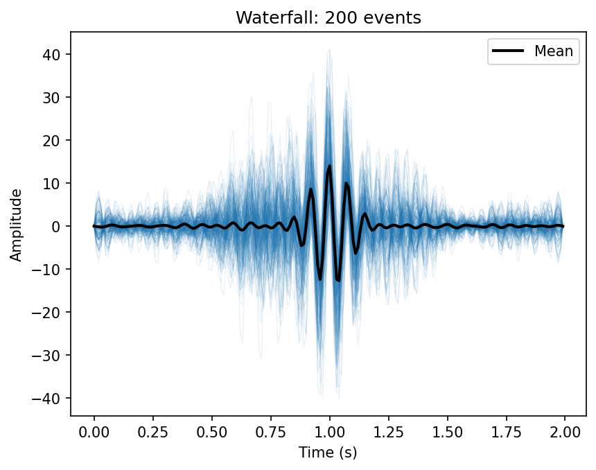
200 sigma-filtered spindle waveforms overlaid, with the population mean in black.
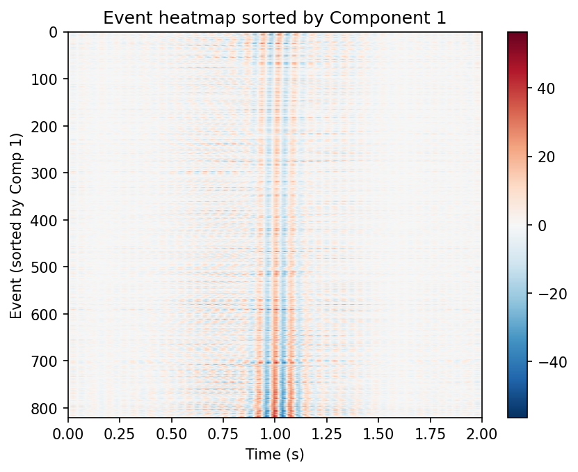
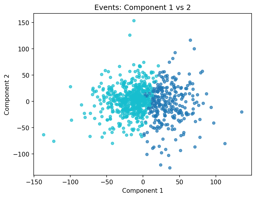
Left: all events sorted by Component 1 loading. Right: k-means clustering in the first two component scores.
Install
pip install subwave
Optional extras:
pip install "subwave[mne]"          # MNE-Python and Luna I/O
pip install "subwave[yasa]"         # YASA spindle detection I/O (pulls in mne)
pip install "subwave[scattering]"   # Wavelet scattering decomposition (kymatio)
pip install "subwave[tensor]"       # Multi-channel tensor decomposition (tensorly)
pip install "subwave[all]"          # All optional backends
Quickstart
import numpy as np
import subwave as sw

rng = np.random.default_rng(0)
t = np.linspace(0, 1, 256)
X = np.stack([np.sin(2 * np.pi * 13 * t) + rng.normal(0, 0.1, 256) for _ in range(100)])

result = sw.decompose(X, method="svd", n_components=5)
result.plot_templates(n=3)
Each template is a basis waveform shape; each loading is how strongly a given event expresses that template. Together they reconstruct the original population.
Or let subwave choose the number of components:
result = sw.decompose(X, n_components="auto")
ECG example
import numpy as np
import subwave as sw

# Stack detected QRS complexes into an event matrix
X_beats = np.load("heartbeats.npy")     # (n_beats, n_samples)
result = sw.decompose(X_beats, method="svd", n_components=3)

# Outlier detection flags ectopic beats
scores = result.outlier_scores()
ectopic = np.where(scores > np.percentile(scores, 99))[0]
Loading data
sw.from_array(X, sfreq=256)                              # plain numpy
sw.from_npz("spindles.npz")                              # Lunascope format
sw.from_mne(epochs)                                       # MNE Epochs
sw.from_yasa(spindles_df, raw_signal, sfreq=256)          # YASA output
sw.from_luna("spindles.txt", "recording.edf", sfreq=256)  # Luna output + EDF
sw.from_edf_batch(["s1.edf", "s2.edf"], channel="C3")     # detect + pool across files
sw.from_lwf("spindles.lwf")                               # Luna .lwf waveform export
from_edf_batch runs a detector (default YASA) on every EDF, extracts windows
around each peak, and returns a single EventMatrix with a .meta DataFrame
recording subject, file, event_index, and peak_sec for each pooled
event.
Luna .lwf files
from_lwf reads Luna's binary .lwf waveform export directly (no optional
dependencies required) and returns an AxisAnnotatedTensor with axes
['instance', 'channel', 'sample'], preserving per-channel labels/units/sample
rates and rich per-event metadata (annotation, instance, anchor and timing
columns):
aat = sw.from_lwf("spindles.lwf")          # a single file
aat = sw.from_lwf(["s1.lwf", "s2.lwf"])    # several files, concatenated
aat = sw.from_lwf("exports/", recur=True)  # every .lwf under a directory

aat.shape                                  # (n_events, n_channels, n_samples)
aat.axis_meta["instance"]                  # per-event DataFrame (id, annot, timing, …)
aat.axis_meta["channel"]                   # label, unit, sr per channel
result = sw.decompose(aat, method="svd", n_components=5)
All files must share the same channel labels and sample rates, and every event
must have the same number of samples (Luna's require=full windows). To inspect
files without loading any signal data, use lwf_summary:
df = sw.lwf_summary("exports/", recur=True)
# One row per file: id, tag, startdate, n_waves, n_channels, channels, srs, …
Decomposition methods
- SVD / PCA (
method='svd') — default, optimal low-rank approximation. Uses randomized SVD for >5000 events. - NMF (
method='nmf') — parts-based, requires non-negative input. - Dictionary learning (
method='dictlearn') — sparse atoms. - Fourier-then-SVD (
method='fourier_svd') — shift-invariant: SVD on per-event magnitude rFFT spectra. Robust to small temporal jitter that corrupts plain SVD. Templates live in frequency space (config['domain'] = 'frequency'). - Scattering-then-SVD (
method='scattering_svd') — locally translation-invariant and stable to deformation via 1-D wavelet scattering (kymatio). Templates live in scattering-coefficient space. Requiressubwave[scattering].
Tensor decomposition (multi-channel)
For 3-D event tensors (n_events, n_samples, n_channels), tensor_decompose
factors temporal and spatial structure separately instead of flattening:
result = sw.tensor_decompose(X, method="cp", rank=3)        # PARAFAC / CP
result = sw.tensor_decompose(X, method="tucker", rank=3)    # Tucker (with core)

result.event_factors        # (n_events, rank)
result.temporal_factors     # (n_samples, rank)
result.spatial_factors      # (n_channels, rank)
result.reconstruction_error # ||X - X_hat|| / ||X||
result.component_waveform(0, channel=1)   # template scaled by channel weight
result.plot()                             # per-component temporal / spatial / loading panels
Requires subwave[tensor].
Working with results
result.templates                        # (n_components, n_samples) basis waveforms
result.loadings                         # (n_events, n_components) per-event scores
result.explained_variance_ratio         # variance captured per component
result.singular_values                  # singular values
result.factor_tables["instance"]        # DataFrame: instance_id, score_1…k, recon_error

result.reconstruct(n_components=3)      # rank-k reconstruction
result.project(new_X)                   # project new events onto learned subspace
result.outlier_scores()                 # per-event reconstruction error
Component selection
k = sw.parallel_analysis(X)             # Horn's parallel analysis
k = sw.elbow(result.singular_values)    # Kneedle elbow detection
k = sw.kaiser(result)                   # Kaiser rule
Spectral characterization
freqs, powers = result.template_spectrum(sfreq=256)
peak_hz = result.template_peak_freq(sfreq=256)     # e.g. [13.2, 11.1] Hz
bw_hz = result.template_bandwidth(sfreq=256)
Clustering
cr = result.cluster(method="kmeans", n_clusters=2)
cr["labels"]                            # cluster assignments
result.cluster_templates(n_clusters=2)  # mean waveform per cluster
Group comparison
perm = sw.permutation_test(X, groups, n_components=3, n_perm=500)
perm.p_value                            # do two groups span different subspaces?

df = sw.comparison.loading_test(result, groups, n_perm=1000)
# Columns: component, observed_diff, p_value, cohens_d, p_corrected
# cohens_d:    standardized effect size (pooled SD)
# p_corrected: Benjamini-Hochberg FDR-adjusted p-values across components
Spindle helpers
Convenience routines for sleep-spindle waveforms (sigma-band filtering, envelope-based alignment, canonical templates).
from subwave.spindles import (
    sigma_filter,             # 9–16 Hz Butterworth bandpass (sosfiltfilt)
    align_by_envelope_peak,   # circularly shift so each event's sigma-envelope peak is centered
    CANONICAL_FAST,           # ~13.5 Hz Gaussian-windowed sinusoid (256 Hz, 1 s)
    CANONICAL_SLOW,           # ~11 Hz   Gaussian-windowed sinusoid (256 Hz, 1 s)
)

X_filt = sigma_filter(X, sfreq=256)
X_aligned = align_by_envelope_peak(X, sfreq=256)
Validation
Tools for checking decompositions against ground truth and for estimating component reliability.
from subwave.validation import (
    synthetic_population,   # generate events from known templates with noise / jitter / amplitude variability
    recovery_score,         # cosine similarity between true and recovered templates (Hungarian-matched)
    cluster_recovery_ari,   # Adjusted Rand Index between true and recovered cluster labels
    bootstrap_stability,    # mean cosine similarity of bootstrap-resampled templates to full-data templates
    split_half,             # template & loading reproducibility on odd/even split
)

# Ground-truth recovery on synthetic data
truth = synthetic_population(templates, n_events=200, noise_std=0.1, random_state=0)
result = sw.decompose(truth["X"], method="svd", n_components=truth["templates"].shape[0])
score = recovery_score(truth["templates"], result.templates)
score["mean_score"]            # cosine similarity (1.0 = perfect)

# Reliability of a real decomposition
boot = bootstrap_stability(X, n_components=3, n_boot=100, random_state=0)
boot["stability_scores"]       # per-component mean similarity across bootstraps

sh = split_half(X, n_components=3, random_state=0)
sh["template_similarity"]      # per-component template reproducibility
sh["loading_correlation"]      # correlation of projected vs native loadings
Serialization
result.save("result.npz")
result = sw.load_result("result.npz")
df = result.to_dataframe()              # flat DataFrame for R/Stata
Plots
result.plot_spectrum()                  # singular value scree plot
result.plot_templates(n=5)              # basis waveforms
result.plot_template_spectra(sfreq=256) # power spectrum of each template
result.plot_scatter(x=0, y=1)           # component 0 vs 1 (supports color= for clusters)
result.plot_heatmap(comp=0)             # events × samples sorted by loading
result.plot_waterfall(n=100)            # overlaid waveforms with bold mean
result.plot_mean_pm(comp=0)             # mean ± component
result.plot_sorted_grid(comp=0)         # events sorted by score
result.plot_residual_hist()             # reconstruction error distribution
result.plot_cumulative_variance()       # cumulative EVR curve
result.plot_reconstruction(event_idx=0) # original vs reconstruction
result.plot_loadings_by_group(groups)   # box/violin by group
result.plot_loadings_over_time(times)   # loading drift across time
See docstrings via help(sw.decompose) for full options, including cluster_sweep, loading_test, subspace_angles, scatter_colored_by, loadings_correlated_with, and more.
Citation
If you use subwave in published work, see CITATION.cff in the repository.
License
MIT
1 maintainer

Metadata
1 maintainer
Release files for subwave 0.4.0
For a detailed explanation of source distributions (sdists) and built distributions (wheels), please see the package formats documentation.
Source distribution (sdist)
| File | Size | Uploaded | |
|---|---|---|---|
| subwave-0.4.0.tar.gz | 1.1 MB | Details |
Built distribution (wheel)
| File | Interpreter | ABI | Platform | Reset |
|---|---|---|---|---|
| subwave-0.4.0-py3-none-any.whl | Python 3 | none | any | Details |
Total release size: 1.2 MB
Release files / subwave-0.4.0.tar.gz
| Download URL | subwave-0.4.0.tar.gz |
|---|---|
| Size | 1.1 MB |
| Tags | Source |
|
SHA-256 checksum How to use checksums |
4d418114d5f8dcf0874976f9807dd181670bb33dff8513ef8bfbd4dbdb186136
|
|
BLAKE2b-256 checksum How to use checksums |
13562503d8d58a4df6af6a26860eb9763b7006064a2b15e61f52faaf453d8117
|
| Upload date | |
|
Uploaded using Trusted Publishing? What is trusted publishing? |
No |
| Uploaded via |
twine/6.2.0 CPython/3.14.6
|
Release files / subwave-0.4.0-py3-none-any.whl
| Download URL | subwave-0.4.0-py3-none-any.whl |
|---|---|
| Size | 48.3 kB |
| Tags | Python 3 |
|
SHA-256 checksum How to use checksums |
5c6b325ffc2e5df4ca9e94cbc072a6e1699fe389aafcc1b04055dc30c348d57e
|
|
BLAKE2b-256 checksum How to use checksums |
871a461648848197c40a1c55361a3ae8845ebe843c3ef5739d9a8568c5b408a4
|
| Upload date | |
|
Uploaded using Trusted Publishing? What is trusted publishing? |
No |
| Uploaded via |
twine/6.2.0 CPython/3.14.6
|














