
swesphere




Shallow-water equations on the sphere with three documented flow regimes: a small geophysical
flow for numerical experiments, verified against the standard test cases and reproducible from a
container. This package is the model only; assimilation filters live in pyteda.
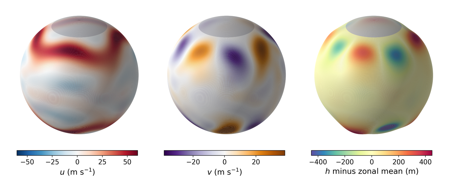
A state of the two_jets record: zonal wind, meridional wind, and the departure of h from its
zonal mean drawn as relief (exaggerated). Polar caps under the sponge are grey. Rendered with
python figures/make_globe3d.py two_jets.
Install
pip install swesphere
Documentation and API: https://aml-cs.github.io/software/swesphere/
Quick start
from swesphere import presets, climatology
model, x0 = presets.two_jets()
S = climatology.build_climatology(model, x0, spinup_days=40, n_snapshots=200, every_days=2)
scales, per_field = climatology.anomaly_scales(model, S)
State vector [u, v, h] (row-major, north to south), model.var_blocks,
model.interior_mask() (outside the polar sponge), model.propagate(x, [t0, t1]).
propagate takes times in seconds and the interval must be a whole number of
time steps. It returns the final state, or the whole trajectory with
just_final_state=False. The spherical-harmonic filter fires on absolute model
time, so splitting a forecast into several calls gives the same answer as one
call: an external driver can choose its forecast window freely without changing
the model. Pass the running time, [t, t + dt_window], not [0, dt_window].
The model
Equations: vector-invariant momentum and flux-form continuity,
du/dt = eta v - (1 / a cos(lat)) dB/dlon        eta = zeta + f,   B = g h + (u^2 + v^2) / 2
dv/dt = -eta u - (1 / a) dB/dlat
dh/dt = -div(h V)
Discretization: regular latitude-longitude (Driscoll-Healy) grid, Nlat = 2 (LMAX + 1),
Nlon = 4 (LMAX + 1) (66 x 132 at the default LMAX = 32); exact zonal derivative by FFT,
second-order centered meridional difference; RK4 in time (dt = 120 s). Dissipation: an
exponential filter in spherical harmonics (pyshtools) applied every filter_every = 3 steps,
and a multiplicative sponge on the wind over the n_pole_rows = 10 rows next to each pole
(poleward of about 63 deg), which is how the model avoids the polar singularity of the grid.
The rows under the sponge are not meant to be used (model.interior_mask()).
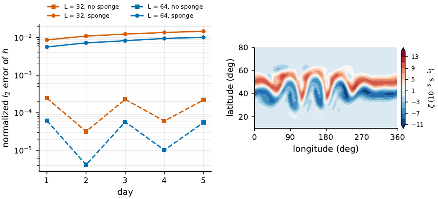
Left: normalized l2 error of h in Williamson test case 2, with and without the polar sponge.
Right: relative vorticity of the Galewsky instability at day 6, LMAX 64 (compare with the
published reference solution).
Two consequences that the experiments quantify:
- The scheme is second order (EXP-00: Williamson test case 2 without the sponge, l2 error of h 2.2e-4 at LMAX 32 and 5.5e-5 at LMAX 64 after 5 days). With the sponge the steady state of that test is disturbed from the polar caps and the error in the interior is about 1e-2.
- The dissipation acts per step, not per second, so the eddy amplitude of a regime depends on
dt * filter_every. The statistics quoted for the presets hold for the defaults (EXP-01).
Presets
| preset | what it is | regime |
|---|---|---|
waves |
solid-body rotation (Williamson TC2) + wave packets (wavenumber 4 north, 3 south), no forcing | quasi-linear Rossby waves on a zonal flow, slowly decaying (no energy source; the filter is the only sink) |
one_jet |
Galewsky jet at 45 N + relaxation of the zonal mean (5 d) | stationary, fairly regular eddies in the north |
two_jets |
Galewsky jets at +-45 deg + the same relaxation | stationary irregular turbulence in both hemispheres; errors advected by the flow |
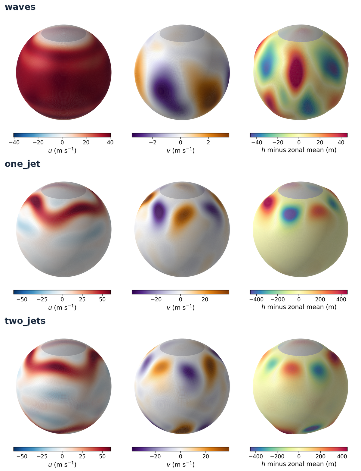
The measured statistics of each regime (eddy std of h, wind, anomaly scales, lag correlations,
first-half against second-half amplitude) are written by EXP-02 to results/EXP-02/regimes.csv.
Measured with the defaults: eddy std of h 8.8 m (waves, decaying), 124 m (one_jet) and
156 m (two_jets); |U|max about 42, 76 and 76 m/s. Note the scales in the figure above: the
meridional wind and the depth anomaly of waves are an order of magnitude weaker than those of
the forced presets.
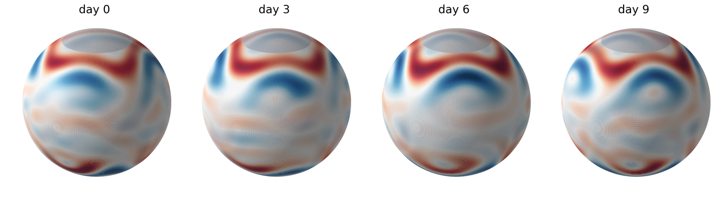
Relative vorticity of the two_jets regime over nine days, starting from a spun-up state. The jet
meanders, sheds eddies and reforms: the flow is chaotic but statistically stationary, which is what
makes it usable as a reference.
The article's experiments (Docker)
docker compose build test
docker compose run --rm test              # unit tests
QUICK=1 docker compose run --rm all       # smoke
docker compose run --rm all               # everything, one core
or detached and in parallel (verification, stability and regimes are independent;
footprint needs regimes; figures needs all):
docker compose run -d verification; docker compose run -d stability; docker compose run -d regimes
docker compose run -d footprint           # when regimes has finished
docker compose run --rm figures           # when everything has finished
| experiment | what it measures | output |
|---|---|---|
exp00_verification.py |
Williamson TC2 error norms (LMAX 32, 64; with and without sponge), Galewsky instability: invariants and vorticity | results/EXP-00/ |
exp01_stability.py |
the stable range of dt for the shipped RK4 (pushed until it blows up) and the eddy amplitude against the filter interval |
results/EXP-01/ |
exp02_regimes.py |
200-state record per preset, per-snapshot series, statistics, stationarity, decorrelation | results/EXP-02/ |
exp03_footprint.py |
balanced against unbalanced perturbations: advection against gravity waves | results/EXP-03/ |
figures/make_figures.py |
figures and tables of the article, one file per panel | results/figures/ |
Besides those, figures/make_globe3d.py <preset> [state.npy] renders the illustrative
three-dimensional views above (it spins the preset up itself if no state is given).
Progress of a detached run: docker ps, docker logs -f <name>; every script logs the preset
and the step, and rewrites its CSV after every case.
Using your own integrator
The package publishes the right-hand side and ships RK4 as the tested stepper. Any other
scheme can be plugged in and runs with the same filter, sponge and forcing (its stable range
of dt is its own: rerun EXP-01):
from swesphere import presets
from swesphere.integrators import INTEGRATORS

def my_step(rhs, u, v, h, dt):          # rhs(u, v, h) -> (du, dv, dh)
    du, dv, dh = rhs(u, v, h)
    return u + dt * du, v + dt * dv, h + dt * dh

INTEGRATORS["mine"] = my_step
model, x0 = presets.two_jets(scheme="mine")
swesphere.dynamics.rhs(u, v, h, grid) is the physics alone; model.rhs(u, v, h) adds the
preset's forcing. swesphere.diagnostics gives mass, energy, potential enstrophy and the
Williamson error norms.
Changes between versions are listed in CHANGELOG.md (0.2.0 fixes the continuity equation of 0.1.0).
Citing, contributing and license
If you use swesphere in your work, please cite it: the CITATION.cff file gives the reference, and
GitHub shows it under "Cite this repository". Bug reports and pull requests are welcome; see
CONTRIBUTING.md. Questions: enino@uninorte.edu.co.
swesphere is released under the MIT license (LICENSE). Its dependencies are NumPy and SciPy
(BSD-3-Clause) and pyshtools (BSD-3-Clause), all compatible with it.
1 maintainer

Metadata
1 maintainer
Release files for swesphere 0.4.0
For a detailed explanation of source distributions (sdists) and built distributions (wheels), please see the package formats documentation.
Source distribution (sdist)
| File | Size | Uploaded | |
|---|---|---|---|
| swesphere-0.4.0.tar.gz | 22.8 kB | Details |
Built distribution (wheel)
| File | Interpreter | ABI | Platform | Reset |
|---|---|---|---|---|
| swesphere-0.4.0-py3-none-any.whl | Python 3 | none | any | Details |
Total release size: 43.1 kB
Release files / swesphere-0.4.0.tar.gz
| Download URL | swesphere-0.4.0.tar.gz |
|---|---|
| Size | 22.8 kB |
| Tags | Source |
|
SHA-256 checksum How to use checksums |
1dfdd8a274271c15b06cd0ac193b9277f01ea619ec56cc1256357aca52195a4c
|
|
BLAKE2b-256 checksum How to use checksums |
4f0680b65431e1688c4d5b5651f445678b329c8efb0a49448e438c3954144b65
|
| Upload date | |
|
Uploaded using Trusted Publishing? What is trusted publishing? |
Yes |
| Uploaded via |
twine/7.0.0 CPython/3.13.14
|
Provenance
Provenance describes where a file came from. On PyPI, provenance is shared via attestations, which provide a verifiable record of the build or publishing details. View details, limitations and caveats.


PyPI Publish Attestation
PyPI verified that this artifact, at this checksum, originated from the publisher listed below.
Signed by GitHub Actions, verified by PyPI on Oct 14, 2026.
Transparency logRelease files / swesphere-0.4.0-py3-none-any.whl
| Download URL | swesphere-0.4.0-py3-none-any.whl |
|---|---|
| Size | 20.2 kB |
| Tags | Python 3 |
|
SHA-256 checksum How to use checksums |
0b827e4db989af01c7da4750883a5db22037c8400e282fb668b7c8e74d49275b
|
|
BLAKE2b-256 checksum How to use checksums |
37bb4c3523f6906763edc9da4c9ebc23170ff50c41309ad525445726eb1ce652
|
| Upload date | |
|
Uploaded using Trusted Publishing? What is trusted publishing? |
Yes |
| Uploaded via |
twine/7.0.0 CPython/3.13.14
|
Provenance
Provenance describes where a file came from. On PyPI, provenance is shared via attestations, which provide a verifiable record of the build or publishing details. View details, limitations and caveats.
PyPI Publish Attestation
PyPI verified that this artifact, at this checksum, originated from the publisher listed below.
Signed by GitHub Actions, verified by PyPI on Oct 14, 2026.
Transparency log













