
Random Forest Enzyme Prediction

Project description
sxlaep: Rapid Enzyme/Non-Enzyme Prediction


sxlaep (Rapid Enzyme/Non-Enzyme Prediction) is an efficient enzyme/non-enzyme prediction tool for protein sequences. It is built on multi-physicochemical property features and the XGBoost machine learning algorithm.
🚀 Features
- Efficient Prediction: Achieves fast and accurate enzyme/non-enzyme classification using optimized feature extraction and the XGBoost model.
- Multi-Mode Support: Supports single-sequence prediction, multi-sequence batch prediction, and FASTA file batch prediction.
- Rich Feature Set: Utilizes multi-physicochemical property pseudo-amino acid composition (Pseudo-AAC), CTD features, and windowed amino acid composition.
- User-Friendly: Offers a concise Python API that is easy to integrate into existing projects.
- Multi-Process Optimization: Employs multi-process parallel processing in the feature extraction step to improve processing efficiency for large-scale datasets.
📦 Dependencies
-
joblib: Used for model saving/loading and parallel processing. -
numpy: Numerical computation. -
pandas: Data processing. -
scikit-learn: Machine learning utilities and evaluation metrics. -
xgboost: Implementation of the gradient boosting tree algorithm.Requirements: Python 3.7 or higher.
📥 Installation
Install from PyPI (Recommended)
pip install sxlaep
Quick start with CLI
sxlaep --input /your_fasta/file.fasta --output /path_to_your_result/result.json
💻 Basic Usage
Import and Initialization
from sxlaep import sxlaep

# Default initialization (uses built-in model)
predictor = sxlaep()

# Initialization with a custom model path (optional)
# predictor = sxlaep(model_path="path/to/your/model.pkl")
Single Sequence Prediction
# Predict a single protein sequence
sequence = "MVLSPADKTNVKAAWGKVGAHAGEYGAEALERMFLSFPTTKTYFPHFDLSHGSAQVKGHGKKVADALTNAVAHVDDMPNALSALSDLHAHKLRVDPVNFKLLSHCLLVTLAAHLPAEFTPAVHASLDKFLASVSTVLTSKYR"

prediction = predictor.predict(sequence)
probability = predictor.predict_proba(sequence)
non_enzyme_prob = 1.0 - enzyme_prob

print(f"Prediction result: {'Enzyme' if prediction == 1 else 'Non-Enzyme'}")
print(f"Prediction probabilities: Non-Enzyme={non_enzyme_prob:.4f}, Enzyme={enzyme_prob:.4f}")
Batch Prediction from FASTA Files
# Batch predict from a FASTA file
fasta_path = "test_sequences.fasta"
results = predictor.predict_fasta(fasta_path)

print(f"Prediction results ({len(results)} sequences):")
for protein_id, result in results.items():
    pred = result['prediction']
    prob = result['probability']
    print(f"{protein_id}: {'Enzyme' if pred == 1 else 'Non-Enzyme'} (Enzyme probability: {prob:.4f})")
📚 API Reference
sxlaep Class
Initialization
sxlaep(model_path=None)
- Purpose: Instantiates the sxlaep predictor, automatically loads the model and initializes feature extraction parameters (e.g.,
LAG=10,W=0.05), ensuring consistency in subsequent prediction workflows. - Parameters:
model_path: Optional. Path to a custom model file. If not provided, the built-inenzyme_xgb_model.pklmodel will be used.
Methods
predict(sequence)
- Purpose: Predicts whether a single protein sequence is an enzyme.
- Parameters:
sequence(String): The protein sequence to be predicted.
- Returns:
prediction(Int): 0 = Non-enzyme, 1 = Enzyme.
predict_proba(sequence)
- Purpose: Predicts whether a single protein sequence is an enzyme.
- Parameters:
sequence(String): The protein sequence to be predicted.
- Returns:
probability(float): Probability of the sequence being an enzyme.
predict_fasta(fasta_path)
- Purpose: Performs batch prediction for protein sequences from a FASTA file.
- Parameters:
fasta_path(String): Path to the FASTA file.
- Returns: Dictionary where keys are protein IDs (from FASTA headers) and values are dictionaries with
prediction(0 for non-enzyme, 1 for enzyme) andprobability(float, enzyme probability).
📝 Notes
- Sequence Format Requirements: Input sequences should only contain single-letter codes (uppercase) for the 20 standard amino acids.
- Sequence Length: The tool automatically processes sequences of different lengths, but excessively short sequences (e.g., < 10 amino acids) may affect prediction accuracy.
- Multi-Process Processing: The feature extraction process uses multi-processing acceleration by default, which automatically adjusts based on the number of CPU cores in the system.
- Model File: Ensure the model file exists and is accessible, especially when using a custom model path.
🌟 Real-World Project Example
sxlaep has been successfully applied in a large-scale marine metagenomics research project. The Marine_Enzyme_Analysis_Pipeline_EN.ipynb notebook demonstrates how to use sxlaep for comprehensive analysis of enzyme sequences from 16,240 Marine Metagenome-Assembled Genomes (MAGs).
Project Highlights:
- Dataset Scale: 33,479,647 predicted protein sequences
- Enzyme Identification: 17,492,382 enzyme sequences identified
- Analysis Scope: Metabolic scaling law, ecological strategies, and biochemical property characterization
1. Parse Prediction Results and Extract Ecological Data
import os
import glob
import numpy as np
import pandas as pd
from tqdm.notebook import tqdm

PRED_DIR = "/path/to/prediction_results"
csv_files = glob.glob(os.path.join(PRED_DIR, "*.csv"))
print(f"Found {len(csv_files)} MAG prediction result files.")

mag_ratios = []
mag_total_seqs = []
mag_mean_probs = []
all_probabilities = []

for f in tqdm(csv_files, desc="Parsing CSVs"):
    df = pd.read_csv(f, usecols=["PredLabel", "Prob_Enzyme"])
    total_seqs = len(df)
    if total_seqs == 0:
        continue

    is_enzyme = (df["PredLabel"] == "Enzyme")
    enzyme_count = is_enzyme.sum()
    ratio = enzyme_count / total_seqs

    if enzyme_count > 0:
        mean_prob = df.loc[is_enzyme, "Prob_Enzyme"].mean()
        sampled_probs = df.loc[is_enzyme, "Prob_Enzyme"].sample(frac=0.01, random_state=42).tolist()
        all_probabilities.extend(sampled_probs)
    else:
        mean_prob = 0.0

    mag_ratios.append(ratio * 100)
    mag_total_seqs.append(total_seqs)
    mag_mean_probs.append(mean_prob)

mag_ratios = np.array(mag_ratios)
mag_total_seqs = np.array(mag_total_seqs)
mag_enzyme_counts = mag_total_seqs * (mag_ratios / 100.0)
mag_mean_probs = np.array(mag_mean_probs)
all_probabilities = np.array(all_probabilities)
2. Ecological Strategy Classification
# Classify MAGs based on enzyme ratio
categories = []
for r_val in mag_ratios:
    if r_val < 40:
        categories.append("Streamlined\n(<40%)")
    elif r_val > 60:
        categories.append("Generalist\n(>60%)")
    else:
        categories.append("Intermediate\n(40-60%)")
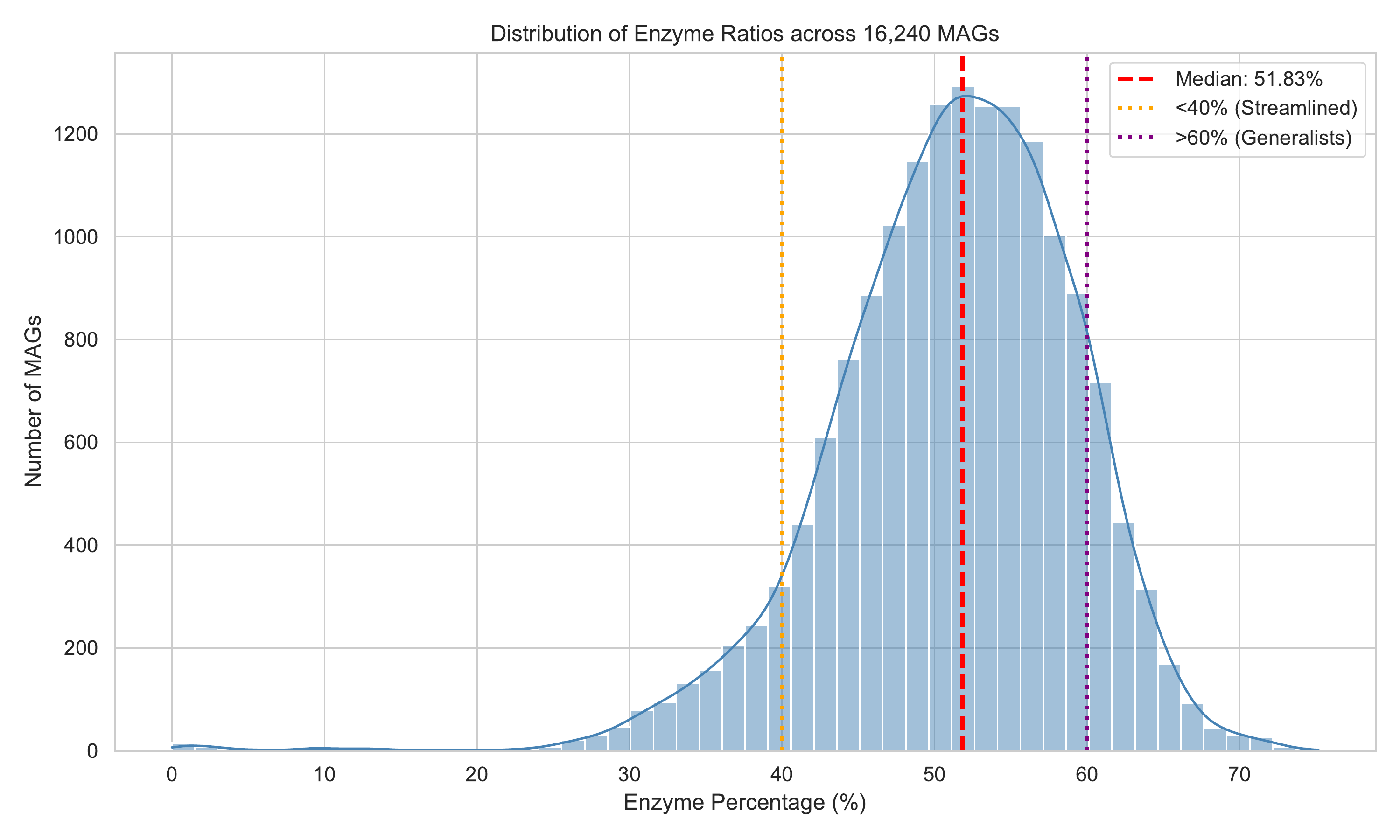
Figure: Distribution of enzyme ratios across 16,240 marine MAGs, revealing three distinct ecological strategies: Streamlined (<40%), Intermediate (40-60%), and Generalist (>60%) genomes.
3. Metabolic Scaling Law Analysis
from scipy import stats

# Calculate Pearson correlation between genome size and enzyme count
r, p_value = stats.pearsonr(mag_total_seqs, mag_enzyme_counts)
p_str = "P < 1e-10" if p_value < 1e-10 else f"P = {p_value:.2e}"

# Linear regression
z = np.polyfit(mag_total_seqs, mag_enzyme_counts, 1)
p = np.poly1d(z)

print(f"Pearson R: {r:.3f}, {p_str}")
4. Prediction Probability Analysis
import seaborn as sns
import matplotlib.pyplot as plt

# Plot probability distribution
sns.histplot(all_probabilities, bins=50, kde=True, color="#3C5488")
plt.axvline(np.median(all_probabilities), color='red', linestyle='dashed',
            label=f'Median: {np.median(all_probabilities):.3f}')
plt.xlabel('XGBoost Probability')
plt.title('Prediction Probability Distribution (Sampled)')
plt.legend()
plt.show()
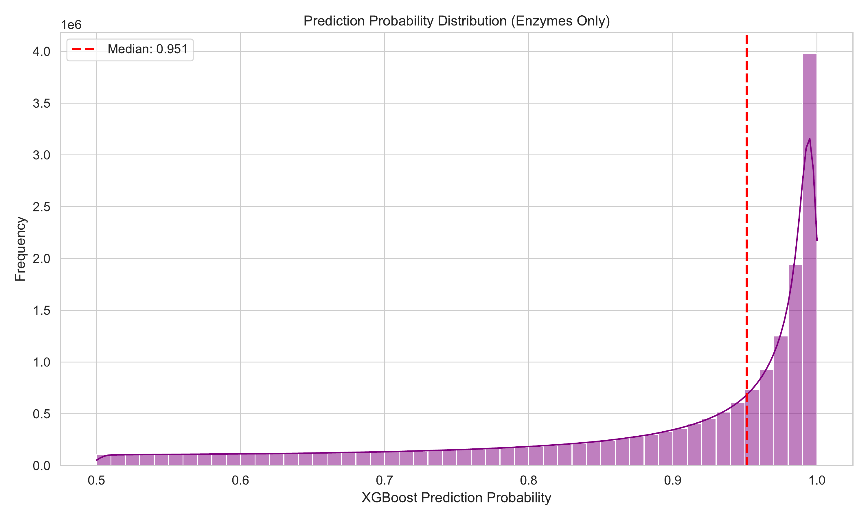
Figure: Distribution of enzyme prediction probabilities, demonstrating the model's confidence in classification.
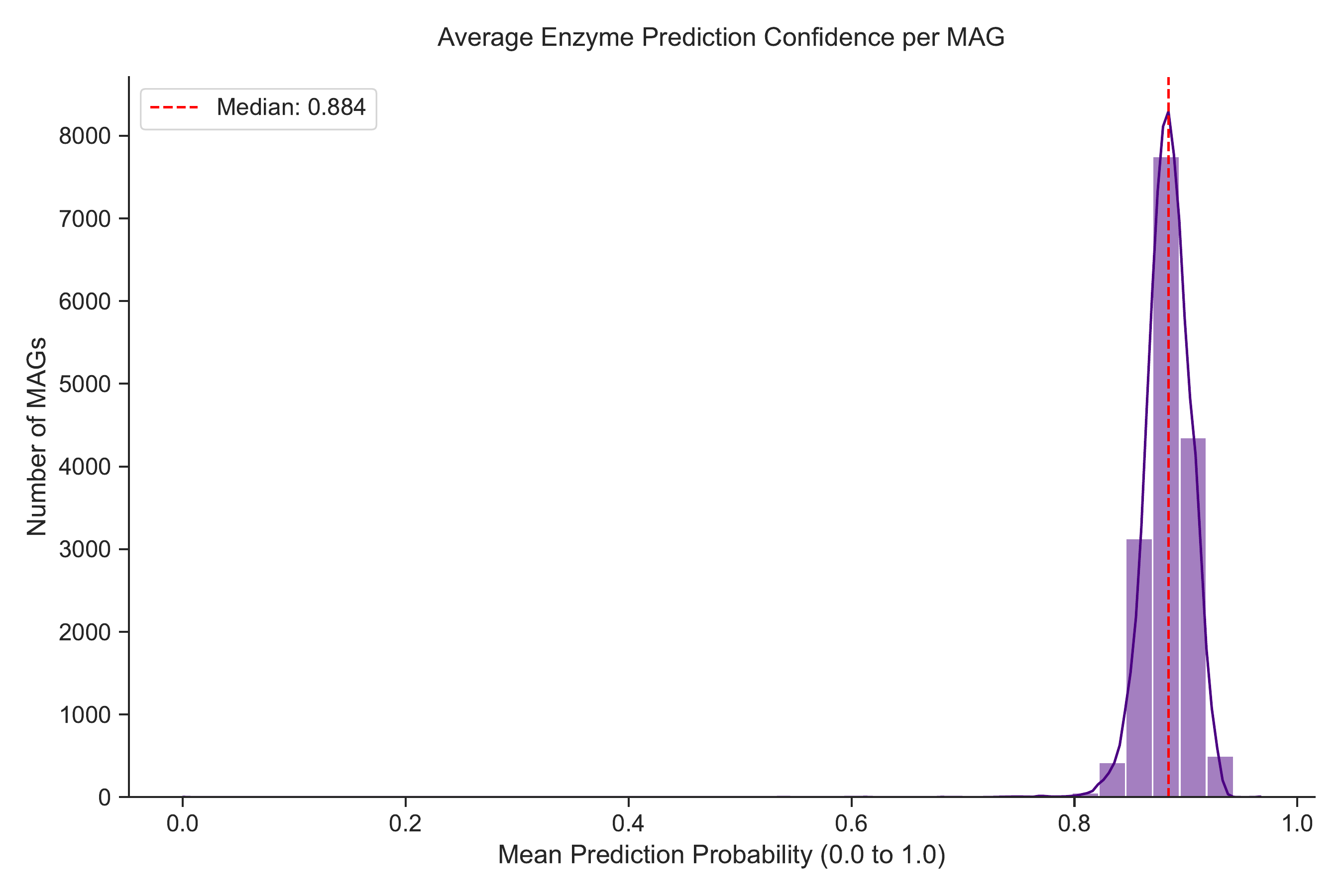
Figure: Distribution of mean prediction confidence across MAGs.
5. Biochemical Properties Calculation (Reservoir Sampling)
import random
from Bio.SeqUtils.ProtParam import ProteinAnalysis

faa_files = glob.glob(os.path.join(PRED_DIR, "*_enzymes.faa"))
SAMPLE_RATE = 100000 / 17500000.0  # Sample ~100k sequences

sampled_seqs = []
lengths = []

def clean_seq(seq):
    return ''.join([aa for aa in seq if aa in "ACDEFGHIKLMNPQRSTVWY"])

for faa in tqdm(faa_files, desc="Sampling FASTA"):
    with open(faa, 'r') as f:
        seq_chunks = []
        for line in f:
            if line.startswith(">"):
                if seq_chunks:
                    seq = "".join(seq_chunks)
                    lengths.append(len(seq))
                    if random.random() < SAMPLE_RATE:
                        sampled_seqs.append(seq)
                seq_chunks = []
            else:
                seq_chunks.append(line.strip())

pis = []
mws = []

for seq in tqdm(sampled_seqs, desc="Computing ProtParam"):
    clean_s = clean_seq(seq)
    if not clean_s:
        continue
    pa = ProteinAnalysis(clean_s)
    try:
        pis.append(pa.isoelectric_point())
        mws.append(pa.molecular_weight() / 1000.0)  # kDa
    except Exception:
        pass
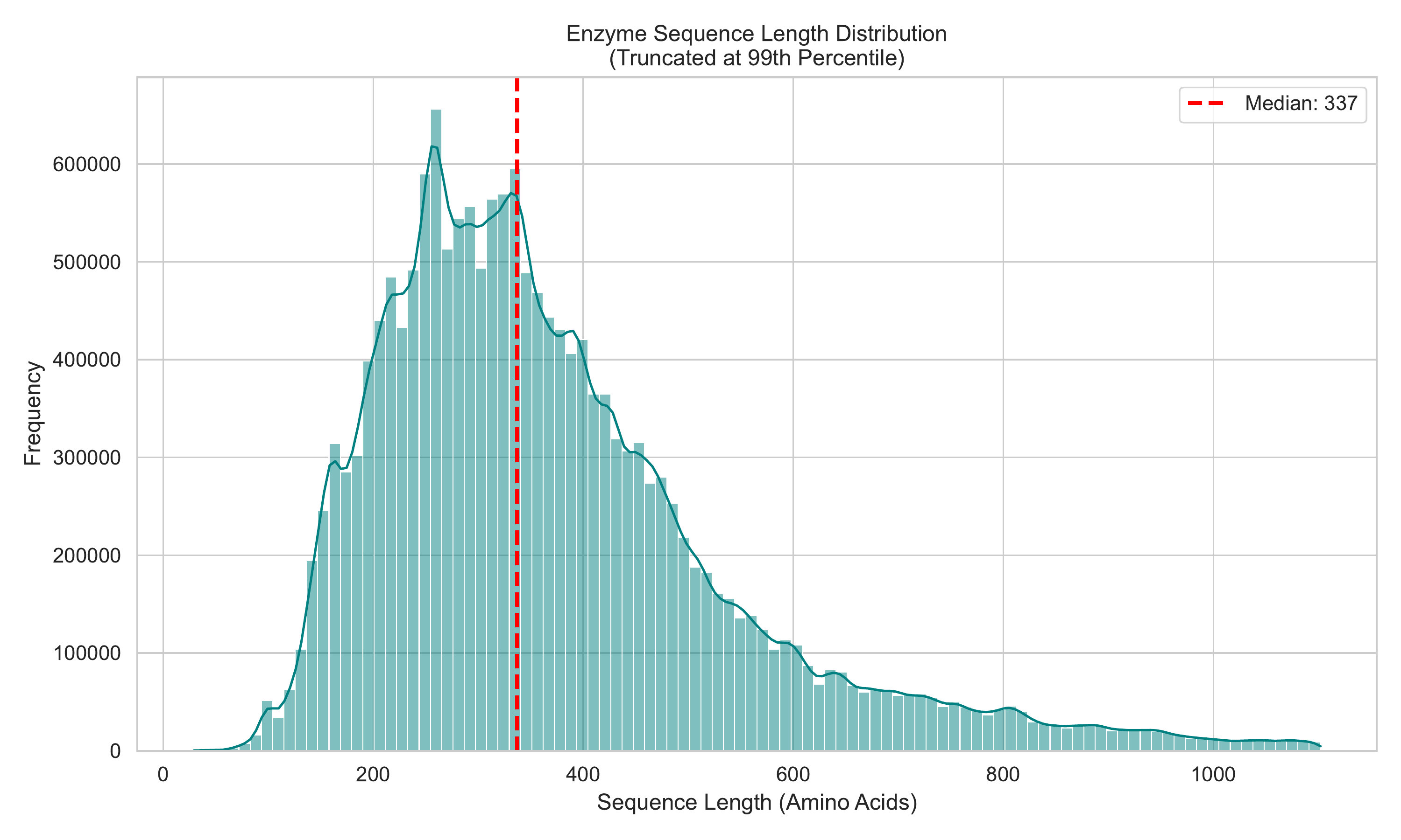
Figure: Length distribution of predicted enzyme sequences from marine metagenomes.
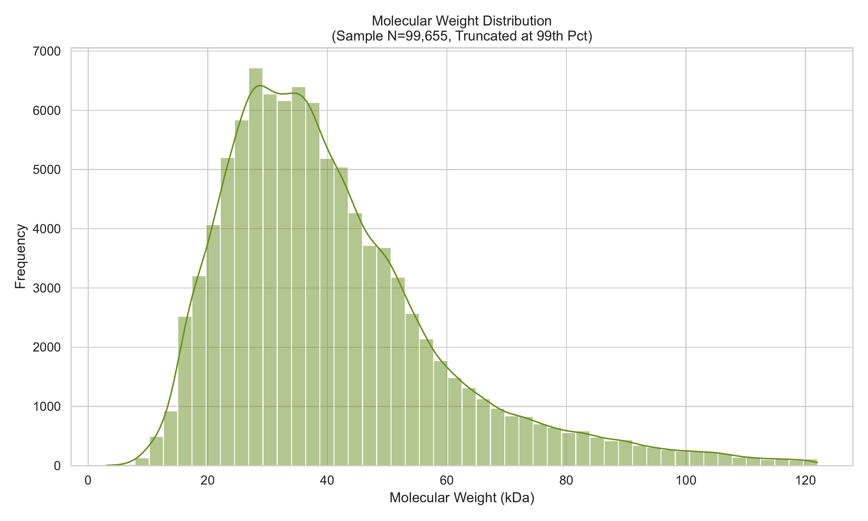
Figure: Molecular weight distribution of predicted enzyme sequences (kDa).
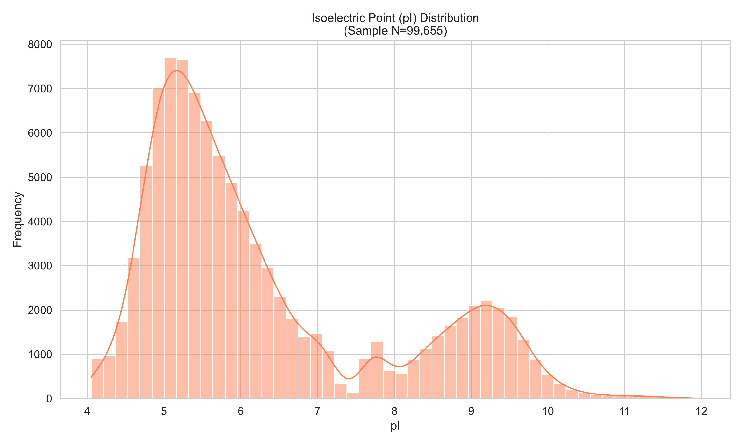
Figure: Isoelectric point (pI) distribution of predicted enzyme sequences.
6. Visualization of Biochemical Properties
fig, axes = plt.subplots(2, 2, figsize=(15, 10))
sns.despine()

# Length Distribution
lengths_arr = np.array(lengths)
p99_len = np.percentile(lengths_arr, 99)
sns.histplot(lengths_arr[lengths_arr <= p99_len], bins=80, kde=True, color="#00A087", ax=axes[0, 0])
axes[0, 0].axvline(np.median(lengths_arr), color='red', linestyle='dashed',
                   label=f'Median: {np.median(lengths_arr):.0f}')
axes[0, 0].set_title('Enzyme Sequence Length Distribution')
axes[0, 0].legend()

# pI Distribution
sns.histplot(pis, bins=50, kde=True, color="#E64B35", ax=axes[1, 0])
axes[1, 0].set_title('Isoelectric Point (pI) Distribution')

# Molecular Weight Distribution
p99_mw = np.percentile(mws, 99)
sns.histplot([m for m in mws if m <= p99_mw], bins=50, kde=True, color="#8491B4", ax=axes[1, 1])
axes[1, 1].set_title('Molecular Weight Distribution')
axes[1, 1].set_xlabel('Molecular Weight (kDa)')

plt.tight_layout()
plt.show()
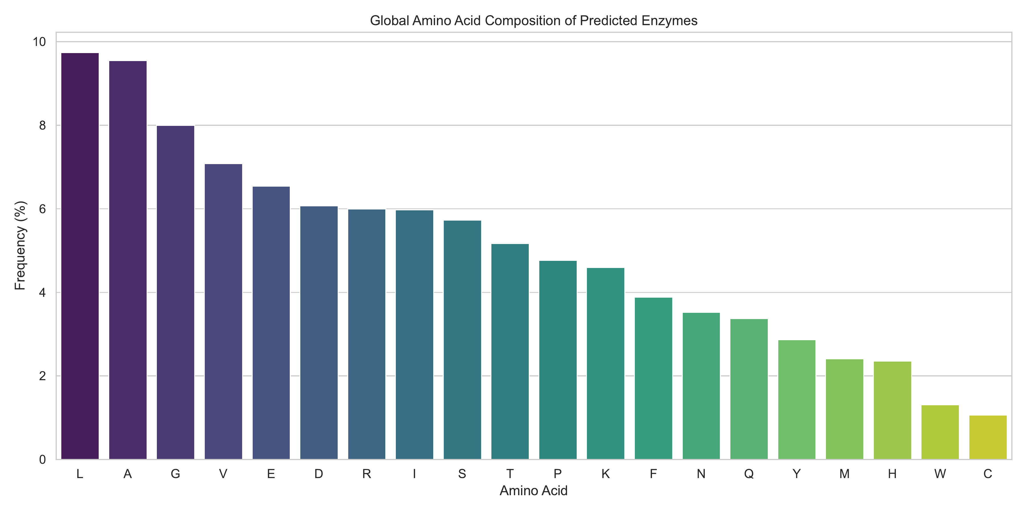
Figure: Amino acid composition analysis of marine enzyme sequences.
The complete analysis pipeline includes:
- Batch prediction using
predict_fasta()for large-scale sequence analysis - Ecological strategy classification based on enzyme ratios (Streamlined/Intermediate/Generalist)
- Metabolic scaling law analysis (genome size vs enzyme count correlation)
- Prediction confidence evaluation for quality assessment
- Biochemical property calculation (pI, molecular weight, amino acid composition)
- Publication-quality figure generation following Science/Nature journal standards
🔧 Troubleshooting
- Failed to import the sxlaep package: Ensure the package is correctly installed in the current Python environment (
pip show sxlaep). - Model loading failure: Verify that the model file path is correct and the file exists at the specified location.
- Prediction errors: Check if the input sequence format is valid and contains only standard amino acid characters.
- Performance issues: For extremely large datasets, consider processing in batches to avoid memory overflow.
🤝 Getting Help
If you encounter any problems, please contact the author:
- Author: DHY
- Email: dhy.scut@outlook.com
📄 License
This project is licensed under the MIT License. See the LICENSE file for details.
🙏 Acknowledgments
The development of this project is supported by several open-source tools, especially machine learning libraries such as XGBoost and scikit-learn.
Version: 1.0.0 | Last updated: 2026


Download files
Download the file for your platform. If you're not sure which to choose, learn more about installing packages.
Source Distribution
Built Distribution
Filter files by name, interpreter, ABI, and platform.
If you're not sure about the file name format, learn more about wheel file names.
Copy a direct link to the current filters
File details
Details for the file sxlaep-1.0.0.tar.gz.
File metadata
- Download URL: sxlaep-1.0.0.tar.gz
- Upload date:
- Size: 6.6 MB
- Tags: Source
- Uploaded using Trusted Publishing? No
- Uploaded via: twine/6.2.0 CPython/3.10.12
File hashes
| Algorithm | Hash digest | |
|---|---|---|
| SHA256 |
cb4c46481b0041599b7a33f152cacecf01454a3b5278cdd338ebf8ae172ea261
|
|
| MD5 |
980446349c4f49f8835cca0e5a5424ce
|
|
| BLAKE2b-256 |
04ab1735f9198da94c557e74fe558eaf08acb6b8d23689cfb8be01c887d17e15
|
File details
Details for the file sxlaep-1.0.0-py3-none-any.whl.
File metadata
- Download URL: sxlaep-1.0.0-py3-none-any.whl
- Upload date:
- Size: 6.7 MB
- Tags: Python 3
- Uploaded using Trusted Publishing? No
- Uploaded via: twine/6.2.0 CPython/3.10.12
File hashes
| Algorithm | Hash digest | |
|---|---|---|
| SHA256 |
64d5f663c3dfd0298ae008f2e0af3111bf4a94e07555a7af73535b33d7d15b3c
|
|
| MD5 |
f2be7b49a738fda16f46ed9e38de5af6
|
|
| BLAKE2b-256 |
bac12566d0856501108d78f249f435784a41cb929cdf55070d533a950c87d3fa
|






