
tareco
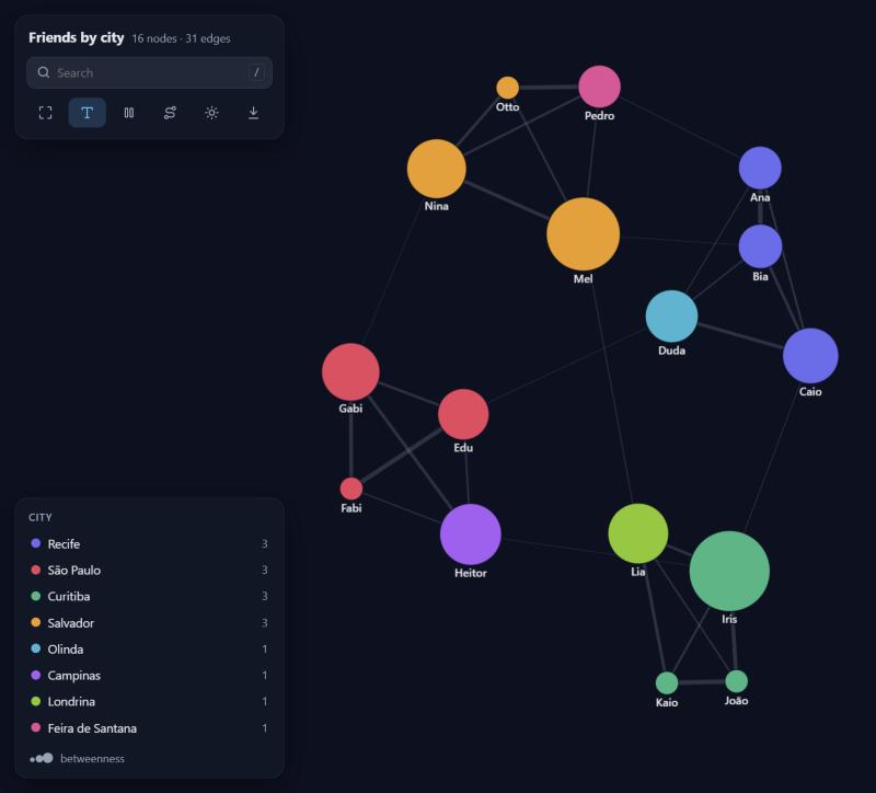
From business data to network answers. Hand it a CSV, a DataFrame or a Spark table and get a beautiful interactive graph you can drag, search and click through, plus what it shows in plain words: which groups exist and what sets each one apart, who bridges them, who concentrates the flow.
No dependencies. Every algorithm is written from scratch in pure Python, and the view is a single self-contained HTML file that works offline.
pip install tareco
New to graphs? There are eight worked recipes, each a real question with its data and a commented script: friends, money transfers, a supply chain, shopping baskets, company e-mail, software dependencies, an outbreak and a subway map. Never used graphs at all? Read the beginner's guide.
One line
import tareco

tareco.show("friends.csv")
That's it. Columns named from/to, source/target, origem/destino
(and friends) are found on their own; otherwise the first two columns are used,
with a tareco.GuessWarning saying which. Every other column becomes an edge
attribute. Nodes are colored by community and sized by importance automatically.
- Weight. A column named
weight,amount,value,quantity,total(orpeso,valor,quantidade...) becomes the strength of each edge; failing that, the only number column (messages,minutes; ids, years and dates do not count). Line widths, the summary andweight="weight"in the algorithms use it. Name another one withweight="minutes". - Repeated pairs add up. Ten rows from ana to bia become one edge with the
numbers summed and
count=10, so a raw log of events works as is.
It also takes whatever you already have:
tareco.show([("ana", "bia"), ("bia", "caio", 3.5)])          # pairs, optional weight
tareco.show({"ana": ["bia", "caio"], "bia": ["davi"]})       # dict of neighbors
tareco.show(df)                                              # pandas or polars DataFrame
tareco.show(spark_df)                                        # Spark DataFrame
tareco.show("friends.csv", nodes="people.csv")               # node attributes too
tareco.show("sales.xlsx")                                    # Excel, no pandas needed
tareco.show(df, source="sender", target="receiver", directed=True)
From the terminal:
tareco friends.csv --nodes people.csv --color city
tareco friends.csv --nodes people.csv --explain --lang pt
tareco orders.csv --directed --max-nodes 20000 -o orders.html
tareco messages.csv --time sent_at --lang pt              # replay over time
tareco messages.csv --around ana --hops 2                 # just the neighborhood of ana
tareco friends.csv --nodes people.csv --report -o friends-report.html
What the network shows
g = tareco.Graph("friends.csv", nodes="people.csv")
g.explain()
What this network shows
- 16 nodes and 31 connections; on average each node connects to 3.9 others.
- Everything is connected in a single network.
- It forms 4 groups that mostly connect among themselves: 77% of the connections stay inside a group.
- Group 1 (4 nodes, 25%): city: Recife in 75% (vs 19% overall). Key members: Bia, Caio and Ana.
- Group 2 (4 nodes, 25%): city: São Paulo in 75% (vs 19% overall). Key members: Gabi, Fabi and Edu.
- ...
- The most important nodes are Gabi, Bia and João.
- Iris is a bridge between groups: it links Group 3, Group 2 and Group 1.
- Mel is a bridge between groups: it links Group 4, Group 3 and Group 1.
- The strongest connection is Ana and Bia (42).
explain() reports the facts worth acting on: separate parts and isolated
nodes, groups and what characterizes each one (attributes that are much more
common, or numbers much higher or lower, than in the whole network), the most
important nodes, bridges between groups, hubs, the most telling patterns (below)
and how concentrated the weight is. Each finding also carries the nodes it talks
about (for f in g.explain(): f.text, f.nodes).
tareco.explain("friends.csv", nodes="people.csv") and tareco.report(...) do
the same straight from a file.
In the interactive view the same findings sit behind the insights button: click one to light up its nodes, or to open that group. The legend shows each group's strongest trait.
g.profile()                     # every group in detail: traits, key members, cohesion
g.profile(groups="segment")     # or group by any attribute, dict or list of sets
tareco.set_language("pt")       # explanations and the interface in Portuguese
                                # (by default: TARECO_LANG, then the computer's language)
Patterns
g.patterns()
- a, b and c form a loop: a to b to c to a. Up to 80 can go all the way around.
- relay receives from 6 nodes and passes almost all of it on to 6 (60 in, 60 out).
- sink receives from 6 nodes but sends to none.
- A chain of 3 intermediaries: c to d to e to f to g.
- x and y send each other similar amounts (50 and 48).
- hub is the only connection of 12 nodes.
Shapes worth a second look, in plain words: loops where things go around and
come back (with how much can make the full turn), fan-in and fan-out,
relays that pass on about what they receive, chains of intermediaries,
back-and-forth pairs, stars and cliques. Loops, fans, relays and
chains need a directed graph. g.patterns(kinds=["cycle"], max_cycle=5) narrows
the search; every pattern has kind, nodes, score and text.
Over time
tl = tareco.timeline(messages, time="sent_at")   # one row per event, any table
tl.explain()
tl.show()                                         # with a time slider and a play button
- From 2026-01 to 2026-06 (6 months): 61 nodes and 467 connections in total.
- The busiest period was 2026-05, with 137 connections.
- 30 new nodes showed up in 2026-04.
- star appeared in 2026-05 with 25 connections at once.
- Two groups merged in 2026-05: the one around p58 and the one around p29.
timeline reads dates, datetimes, ISO text, dd/mm/yyyy or mm/dd/yyyy (worked
out from the data) and plain numbers, and picks days, weeks, months, quarters or
years so there are at most 24 periods (freq= to choose). It reports activity
jumps and drops, waves of newcomers, nodes whose connections suddenly jump,
groups that form, merge or split, and quiet periods.
tl["2026-05"]               # the network of one period (a Graph)
tl.union                    # everything, with first/last period on each edge
tl.activity()               # nodes, connections and weight per period
tl.spread("ana")            # who could have heard from ana, following events in order
tareco.timeline(rows, time="day", cumulative=True, weight="amount")
In the view, the slider replays the periods; clicking a dated insight jumps to its period.
Around a node, in huge tables
near = tareco.neighborhood(spark.table("chat.messages"), start="ana", hops=2,
                           source="sender", target="receiver")
near.show(color="hop")
When a table is far too big to load, start from the nodes you care about and
grow outward. With Spark every hop is a query that runs in the cluster (a
broadcast join when the frontier is large); only the matching edges come back.
It also works on pandas DataFrames, CSV files and rows. max_nodes (5,000) caps
the growth, keeping the most connected nodes of the last hop.
Reports and tables
g.report("friends-report.html")               # findings, group and node tables, the graph
tl.report("messages-report.html")             # plus activity per period and the slider
nodes, edges = g.to_pandas(metrics=["pagerank", "community", "degree"])
nodes, edges = g.to_spark(spark, metrics=["community"])   # back to the lakehouse
g.explain().to_pandas(), g.profile().to_pandas(), g.patterns().to_pandas()
The report is one self-contained HTML file to send to someone who will never open a notebook.
Two-sided data
Business data often says "customer bought product" or "account used device", not
"who is linked to whom". project links the things you care about through what
they share:
purchases = spark.table("sales.items")          # customer, product, amount, segment
g = tareco.project(purchases, nodes="customer", via="product")
g.explain()                                     # customer groups and what they buy alike

items = tareco.project(purchases, nodes="product", via="customer")
items.top_neighbors("diapers", n=3)             # bought together, most shared customers first
Edges get weight (shared products), shared and a few examples. Columns that
never change for a customer (like segment) become customer attributes, and
changing numbers are summed (amount_total), so groups can be profiled right away.
method="jaccard"scores pairs by overlap (0 to 1);method="newman"lets popular products count less, so "both bought water" means little.- Products bought by more than
max_item_sizecustomers (1,000) are skipped with a warning: they link everyone to everyone and cost millions of edges. attrs=customers_dfbrings a table of customer attributes along.g.project(nodes)does the same for a graph that already holds both sides.
The view
- Hover a node to light up its neighborhood; click it for a side panel with its metrics, attributes and clickable neighbors.
- Drag nodes around; dragged nodes stay pinned (right-click to release).
- Search with
/, jump with Enter. - Shortest path mode: click two nodes and the route lights up.
- Legend filters: click a group to hide it, double-click to see only it.
- Freeze the layout, toggle labels, switch dark/light, save a PNG.
- Directed graphs get arrows;
particles=Trueanimates the flow. dim=3gives you a 3D graph you can orbit.
g.show(
    color="city",            # attribute or metric: "community", "pagerank", "degree",
                             # "betweenness", "closeness", "clustering", "core", "component"
    size="betweenness",      # same options, numbers only
    label="name",            # attribute to display instead of the id
    edge_width="messages",   # defaults to "weight" when edges have one
    title="Friends",
    theme="dark",            # "auto", "dark", "light"
)
g.save("friends.html")       # standalone file, send it to anyone
color and size also accept a {node: value} dict (like the output of any
algorithm), a function of the node, or a fixed CSS color.
Notebooks and Databricks
In Jupyter, VS Code, Colab and Databricks, g.show() draws the graph right in
the cell, and so does leaving a graph as the last line of a cell. On Databricks
it goes through displayHTML. Where there is neither a notebook nor a browser
(a cluster job, a server), the page is saved to a temporary file and its path is
printed.
Notebook output is kept under a size budget, because big outputs get cut:
Databricks truncates cell output at 10 MB by default (DBR 17+). If a graph does
not fit, tareco keeps its most important part and says so in the header
(48,000 of 1,200,000 nodes). Pass budget_mb= to change it; on Databricks,
%set_cell_max_output_size_in_mb 20 raises the limit.
Checking an environment
tareco.doctor(spark) # or tareco.doctor() without Spark; `tareco --doctor` in a terminal
OK    environment                 tareco 1.3.0, Python 3.12.3, Databricks 17.3, notebook output budget 9 MB
OK    webgl page                  20,000 nodes, 2.0 MB, ASCII only
OK    notebook output             60,000-node graph fits in 5.1 MB (budget 9 MB)
OK    spark: flavor               Spark Connect, Spark 4.0.1
OK    spark: neighborhood (join)  57 nodes within 2 hops of 'hub'
...
tareco doctor: all good
It runs every path that can break in a new place (notebook detection, output size, the WebGL and canvas pages, timelines, reports and, given a session, reading from Spark, neighborhoods, exports and timelines there, classic Spark or Spark Connect) and reports each one. For Databricks there is a ready notebook, examples/databricks_check.py: import it, run all, and every cell after the doctor should draw a graph.
Spark
from pyspark.sql import functions as F

messages = spark.table("chat.messages")        # sender, receiver, sent_at, ...

edges = (messages
         .groupBy("sender", "receiver")
         .agg(F.count("*").alias("weight")))

g = tareco.Graph(edges, source="sender", target="receiver", directed=True)
g.show(title="Who talks to whom")
A Spark DataFrame is streamed to the driver one partition at a time (no pandas
needed), and DECIMAL columns become floats. Anything above max_rows rows
(1,000,000 by default) is refused with a hint to aggregate in Spark first, which
is almost always the right move: a graph of who-pays-whom with a total per pair
is far smaller than the raw transactions. max_rows=None lifts the limit.
Big graphs
Tens of thousands of nodes are fine. The view changes strategy as the graph grows:
- Up to 2,000 nodes / 8,000 edges: the canvas view above, animated.
- Bigger: a WebGL view (sigma.js). The layout runs in a background worker, so the page never freezes while it settles, and edges fade with density so structure shows instead of a white blob. Nodes are pulled toward their community, so groups read as islands.
- Group overview: every community (or every value of a categorical
color) becomes one bubble, sized by members and linked by how much they interact. Click a bubble to open just that group; very big graphs open here first. - Trimming: past
max_nodes(50,000) ormax_edges(200,000), only the most important nodes (by PageRank) and the heaviest edges are embedded. The overview still counts everything.
g.show(renderer="webgl")              # force a renderer: "auto", "canvas", "webgl"
g.show(max_nodes=20_000)              # embed less (smaller, faster page)
g.betweenness(k=500)                  # estimate from 500 sources instead of all nodes
Exact betweenness needs a search from every node. With the optional igraph
package installed (pip install igraph), it runs there for graphs above 1,000
nodes, about 15 times faster; tareco itself stays dependency-free.
Community detection handles 50,000 nodes and 200,000 edges in about two seconds, in pure Python.
The graph
g = tareco.Graph("friends.csv", nodes="people.csv")

g.add_edge("Ana", "Zeca", weight=2, since=2019)
g.add_node("Zeca", city="Recife")

g.nodes["Ana"]              # {'city': 'Recife', 'age': 31}
g.edges["Ana", "Bia"]       # {'messages': 42}
g.neighbors("Ana")          # ['Bia', 'Caio', 'Duda', 'Pedro', 'Zeca']
g.degree("Ana")             # 5
len(g), g.edge_count        # (17, 32)

g.subgraph(["Ana", "Bia", "Caio"])
g.ego("Ana", radius=2)       # everyone within two steps
g.reverse(), g.to_undirected(), g.copy()
The questions
| Ask | Method |
|---|---|
| What it shows, in words | g.explain(), g.profile() |
| Overview numbers | g.summary() |
| Shortest route | g.shortest_path(a, b, weight=None), g.distance(a, b), g.distances(a) |
| Who is important | g.pagerank(), g.degree_centrality() |
| Who bridges groups | g.betweenness(k=None) (k sources estimate it fast) |
| Who is close to everyone | g.closeness() |
| Which groups exist | g.communities() (Louvain), g.modularity(groups) |
| Are they connected | g.components(), g.strong_components(), g.is_connected() |
| How tight is it | g.clustering(), g.triangles(), g.transitivity(), g.density() |
| The core | g.core_number(), g.k_core(k) |
| Who should meet | g.suggest_links(node=None, top=10) (Adamic-Adar) |
| Strongest ties of a node | g.top_neighbors(node, n=5) |
| Cheapest wiring | g.spanning_tree(weight="weight") |
| How much can flow, and the bottleneck | g.max_flow(a, b, capacity="weight") (.value, .flows, .cut) |
| Alternative routes | g.k_shortest_paths(a, b, k=3, weight=None) |
| Shapes worth a look | g.patterns() |
| Order of tasks | g.topological_sort(), g.has_cycle(), g.find_cycle() (one loop, any length) |
| Size of the world | g.diameter() |
| Walk it | g.bfs(a), g.dfs(a) |
Results are plain dicts, lists and sets. Pass weight="some_attribute" to use
edge weights. The algorithms are tested against networkx and give the same
numbers.
Ready-made graphs
tareco.community_graph([30, 20, 10])   # planted groups, great for testing communities()
tareco.scale_free_graph(500, 2)        # a few big hubs, like the web
tareco.small_world_graph(100, 4, 0.1)  # ring with shortcuts
tareco.random_graph(100, 0.05)
tareco.grid_graph(10, 10), tareco.complete_graph(8), tareco.star_graph(6)
tareco.path_graph(5), tareco.cycle_graph(5)
In and out
g.to_csv("edges.csv", "nodes.csv")    tareco.read_csv("edges.csv", "nodes.csv")
g.to_json("graph.json")               tareco.read_json("graph.json")
                                      tareco.read_excel("book.xlsx", sheet="sales")
nodes_df, edges_df = g.to_pandas()    tareco.Graph(df, nodes=nodes_df)
g.to_networkx()                       tareco.Graph(nx_graph)
CSV files may use , ; \t or |, and 1,5-style decimals are understood.
.xlsx files are read without pandas or Excel: dates become dates, numbers numbers.
Development
pip install -e ".[test]"
pytest
The interactive views are drawn with force-graph, sigma.js and graphology (all MIT), bundled inside the package so pages work offline. The 3D view loads 3d-force-graph from a CDN.
1 maintainer

Metadata
1 maintainer
Release files for tareco 1.3.0
For a detailed explanation of source distributions (sdists) and built distributions (wheels), please see the package formats documentation.
Source distribution (sdist)
| File | Size | Uploaded | Provenance | Actions |
|---|---|---|---|---|
| tareco-1.3.0.tar.gz | 261.4 kB | With provenance | Details for tareco-1.3.0.tar.gz |
Built distribution (wheel)
| File | Interpreter | ABI | Platform | Actions Reset |
|---|---|---|---|---|
| tareco-1.3.0-py3-none-any.whl | Python 3 | none | any | Details for tareco-1.3.0-py3-none-any.whl |
Total release size: 495.5 kB
Release files / tareco-1.3.0.tar.gz
| Download URL | tareco-1.3.0.tar.gz |
|---|---|
| Size | 261.4 kB |
| Tags | Source |
|
SHA-256 checksum How to use checksums |
782f06528701fea89dad0e3f672e70c0d0cdb62df2b2f54dbf3e9d47c8f9253f
|
|
BLAKE2b-256 checksum How to use checksums |
7647f3e63a8265b88a6f6bb6014e34254363b9893cc2dad984afde77b8503a03
|
| Upload date | |
|
Uploaded using Trusted Publishing? What is trusted publishing? |
Yes |
| Uploaded via |
twine/7.0.0 CPython/3.13.16
|
Provenance
Provenance describes where a file came from. On PyPI, provenance is shared via attestations, which provide a verifiable record of the build or publishing details. View details, limitations and caveats.


PyPI Publish Attestation
PyPI verified that this artifact, at this checksum, originated from the publisher listed below.
Signed by GitHub Actions, verified by PyPI on Oct 22, 2026.
Transparency logRelease files / tareco-1.3.0-py3-none-any.whl
| Download URL | tareco-1.3.0-py3-none-any.whl |
|---|---|
| Size | 234.0 kB |
| Tags | Python 3 |
|
SHA-256 checksum How to use checksums |
cfe3a6e6a362115027881c18cdbf95e59e866f325ba6d5dfb676a33a1b7f8438
|
|
BLAKE2b-256 checksum How to use checksums |
60c16cb0736ae8471d949a794463ad0e30c2ceced1de7eee980b45a317a80025
|
| Upload date | |
|
Uploaded using Trusted Publishing? What is trusted publishing? |
Yes |
| Uploaded via |
twine/7.0.0 CPython/3.13.16
|
Provenance
Provenance describes where a file came from. On PyPI, provenance is shared via attestations, which provide a verifiable record of the build or publishing details. View details, limitations and caveats.
PyPI Publish Attestation
PyPI verified that this artifact, at this checksum, originated from the publisher listed below.
Signed by GitHub Actions, verified by PyPI on Oct 22, 2026.
Transparency logSecurity for tareco 1.3.0
Provenance
Provenance describes where a file came from. On PyPI, provenance is shared via attestations, which provide a verifiable record of the build or publishing details. View details, limitations and caveats.
Full provenance
Both files in this release have been uploaded with provenance metadata.
Attestation for tareco-1.3.0.tar.gz
PyPI Publish Attestation
PyPI verified that this artifact, at this checksum, originated from the publisher listed below.
Signed by GitHub Actions, verified by PyPI on Oct 22, 2026.
Transparency logA note on package security
PyPI is a repository for distributing packages, not a service for auditing them. While third-party security researchers and our staff do their best to detect and remove malicious packages, PyPI cannot guarantee the quality, security or suitability of any given package.
To learn more about protecting yourself from malicious actors, visit our package security documentation.














