
TopoPPI
TopoPPI helps you explore where two proteins meet. Open a PDB or mmCIF structure, choose a pair of chains, and view their interaction surface as a 2D atlas or an interactive 3D interface.
Highlight residues, inspect their contacts, and color the interface with your own numerical data. Save an editable atlas to return to your work, or export figures as PNG, TIFF, SVG or PDF. The desktop app, command line and Python API use the same mapping and annotation tools.
Get started: Windows · macOS · Linux · Command line · Python API
Example outputs
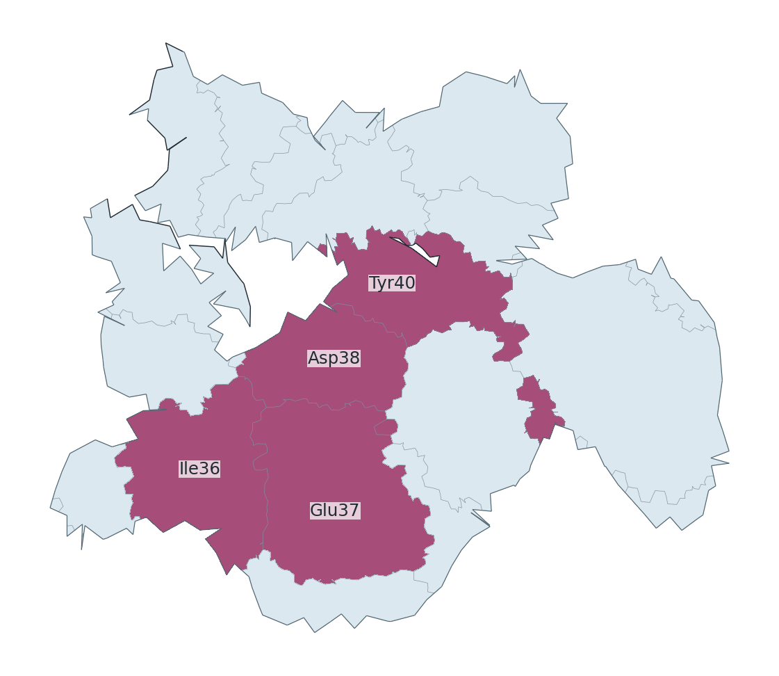
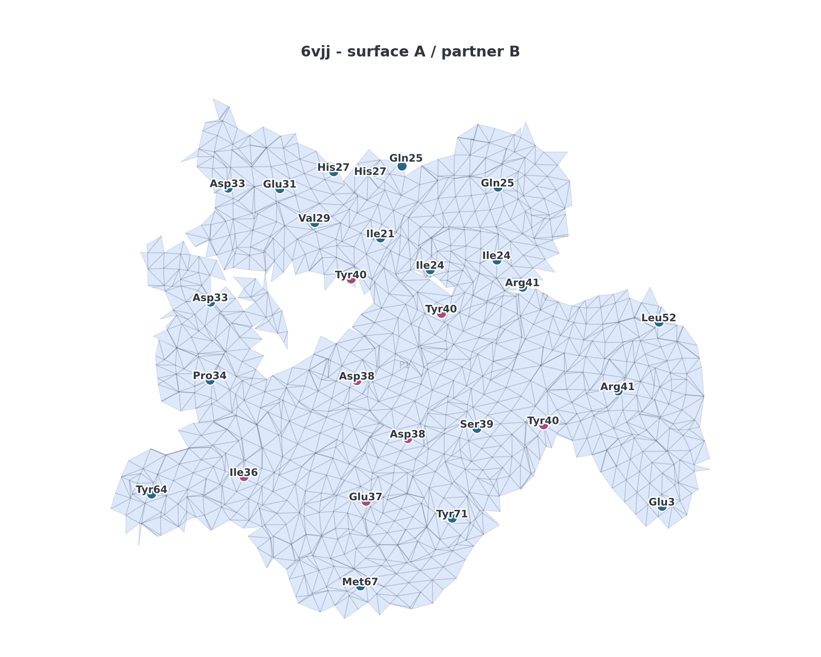
These four outputs show the same KRAS–RAF1 interface (PDB 6VJJ, surface chain A, partner chain B). Magenta highlights Ile36, Glu37, Asp38 and Tyr40 in the first three views.
| 2D residue footprints | 3D interface |
|---|---|
 |
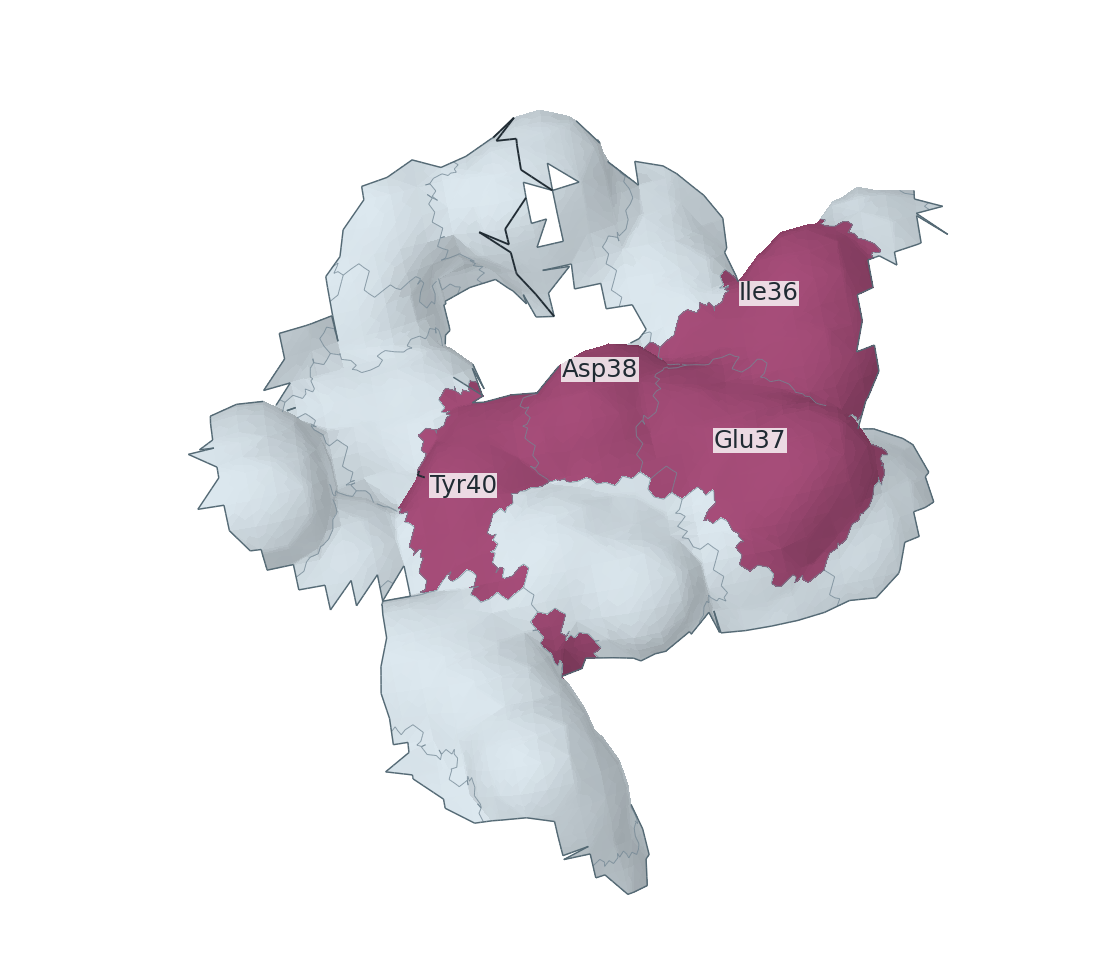 |
| See the full interface and the area occupied by each residue. | Follow the surface shape while retaining the same residue annotations. |
| Residue markers | Numerical annotations |
 |
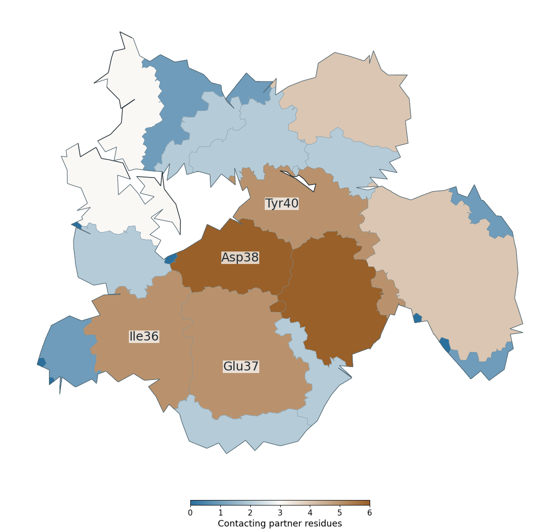 |
| Locate contacting residues and follow their labels across the map. | Load a CSV file to map your values onto residue regions. |
The numerical example counts contacting partner residues using a 6 Å heavy-atom distance cutoff. See the Residue footprints guide for CSV formatting and the 3D interface guide for camera and display controls.
Choose a starting point
| Your goal | Start here |
|---|---|
| Make a first map on Windows | Install the Windows app and use the Basic page |
| Make a first map on a Mac | Install the macOS app and use the Basic page |
| Use Linux or automate one structure | Install with Conda and pip and run topoppi |
| Call TopoPPI from Python | Python API |
| Inspect a saved atlas in three dimensions | 3D interface view |
| Compare methods across a dataset | Benchmark a dataset |
| Reproduce a publication study | Publication workflow tools |
Install TopoPPI
Choose the TopoPPI 2.1 package for your operating system below.
Windows
Download the 64-bit Windows installer:
TopoPPI-2.1-windows-x86_64-setup.exe
Get the installer from the v2.1 release. Open it and keep its setup window open while it creates the private environment. A fresh installation commonly takes 5–15 minutes and uses GitHub, conda-forge, and PyPI. After setup, open TopoPPI GUI from the Start Menu. Routine analysis of local structures can run offline.
The current installer is unsigned, so Windows SmartScreen may ask you to confirm the file. Download it from the project release page, select More info, then select Run anyway. Upgrade, repair, removal, and local build instructions are in the Windows guide.
macOS
Download the disk image for your Mac's architecture:
TopoPPI-2.1-macos-arm64.dmg       Apple Silicon
TopoPPI-2.1-macos-x86_64.dmg      Intel
Get the disk image from the v2.1 release. Open it, drag TopoPPI to Applications, and open the app. The app uses ad-hoc signing. If macOS blocks it, open System Settings > Privacy & Security, choose Open Anyway for TopoPPI, and confirm Open. Older macOS releases may also offer Open through the app's Control-click menu. Keep the preparation window open while the bundled runtime expands. Later launches reuse that runtime.
The app includes Python, scientific dependencies, and native OptCuts, and supports macOS 12 or later. Startup recovery, upgrades, removal, and local build instructions are in the macOS guide.
Linux
TopoPPI uses Python 3.10. Create an environment, install version 2.1 from PyPI, and launch the desktop app:
conda create -n topoppi -c conda-forge \
  python=3.10 tk igl=2.6.* numpy scipy biopython scikit-image \
  matplotlib trimesh networkx pillow rtree shapely \
  mdanalysis rdkit psutil tqdm meshio pip
conda activate topoppi
python -m pip install "topoppi[all]==2.1"
topoppi-install-optcuts
command -v OptCuts_bin
topoppi-gui
topoppi-install-optcuts downloads the Linux x86-64 executable matching the installed release. Other Linux architectures use a locally built executable through TOPOPPI_OPTCUTS_BIN. To work from a source checkout, install with python -m pip install ".[all]" and use bash tools/OptCuts/install_optcuts.sh from the repository root.
Create an interface map
Desktop app
Launch topoppi-gui, or open the installed application on Windows or macOS.
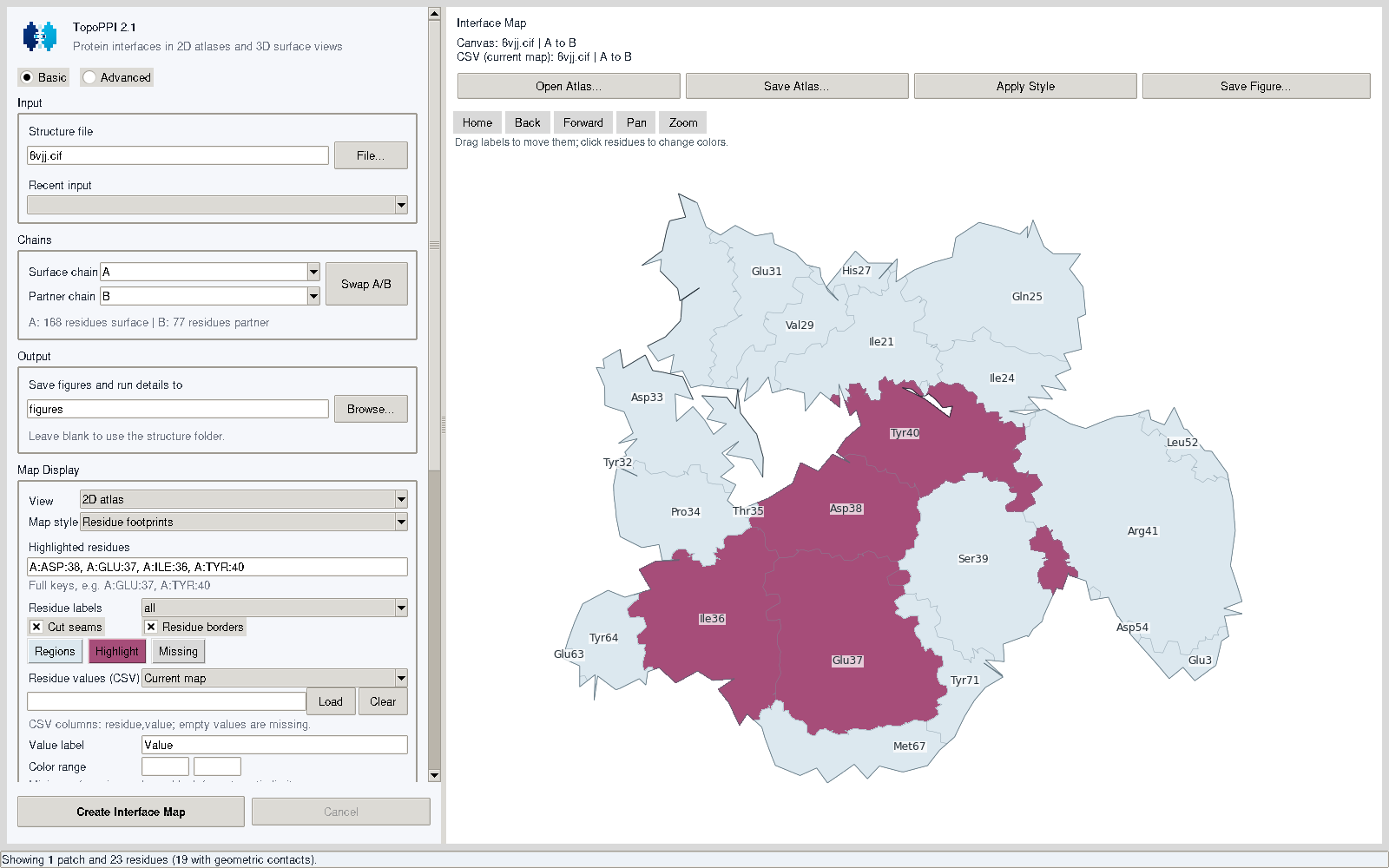
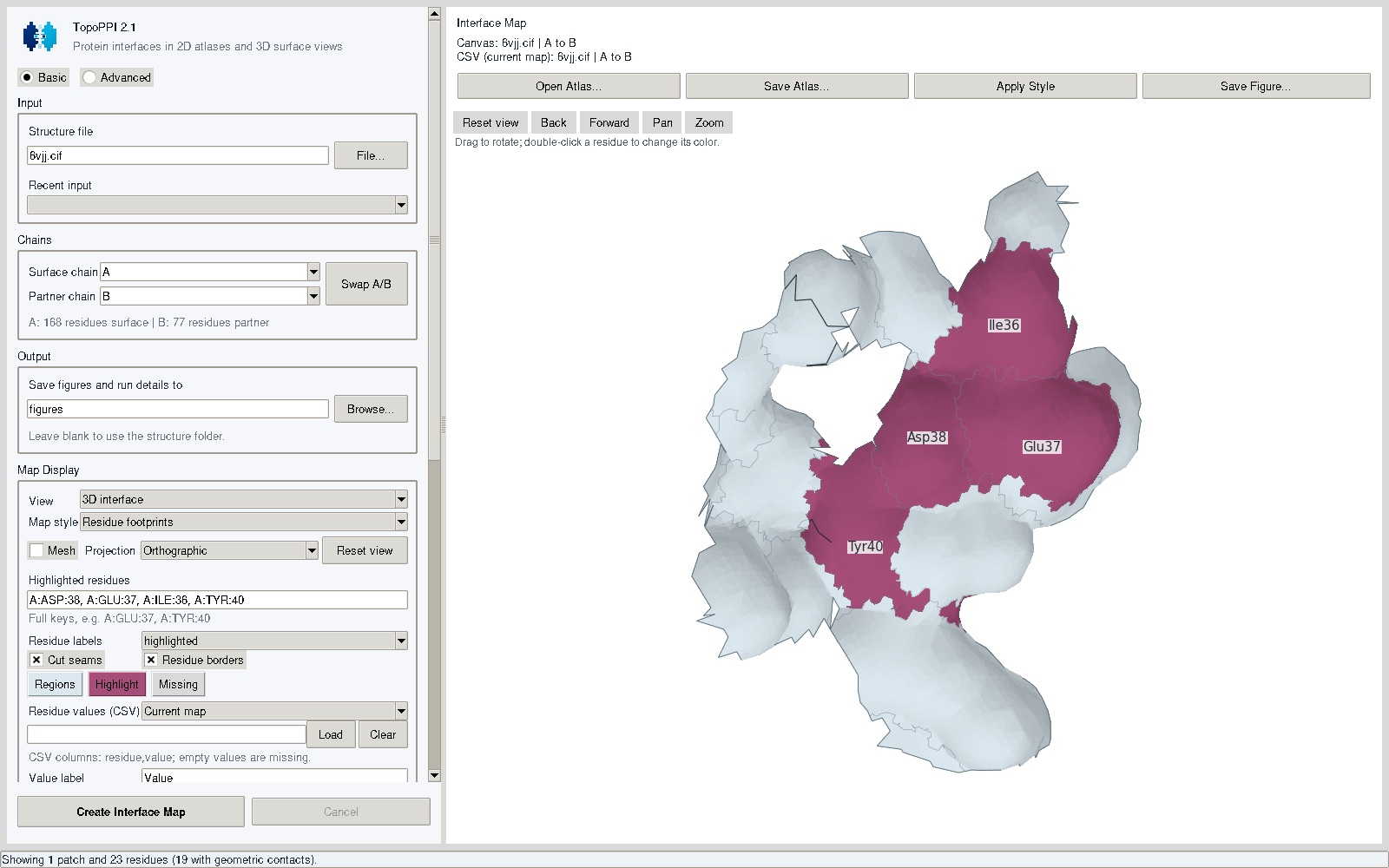
Desktop screenshots: 2D atlas and 3D interface
2D atlas: inspect residue regions and adjust labels, highlights and colors.
3D interface: rotate the surface and save the view for later editing or export.
- On Basic, choose a
.pdb,.cif, or.mmcifstructure. - Review the detected protein chains and residue counts.
- Set Surface chain to the protein whose surface you want to map.
- Set Partner chain to the contacting protein. Swap A/B maps the opposite surface.
- Choose the output folder and interaction types.
- Select Create Interface Map.
Once the result appears, choose 2D atlas or 3D interface under View. Use Map style to switch between residue markers and filled residue footprints. Save Atlas keeps the result editable; Save Figure exports the current view.
TopoPPI generates ProLIF annotations when no interaction JSON is supplied. The completed run writes the image, its .topoppi.json run record, and the generated .prolif.json file to the chosen output folder. Advanced settings expose the surface, topology, UV, OptCuts, labeling, and export controls.
The Help menu shows the installed version and opens the user guide or issue tracker. During a run, the status area reports Load, Surface, Patch, OptCuts, and Render progress.
The map panel identifies the structure and chain pair it displays. Preparing another input leaves the current atlas available for editing and saving. Once computation finishes, display settings can be adjusted with Apply Style using the calculated atlas.
Command line
The shortest command is:
topoppi path/to/complex.pdb \
  --chain-a A \
  --chain-b B \
  --output interface_map.png
This creates:
interface_map.png
interface_map.topoppi.json
complex.A-B.prolif.json
The generated ProLIF file is placed beside the output image. Supply an existing file with --prolif interactions.json when interaction evidence has already been prepared.
For a Linux x86-64 source checkout, this small smoke run uses the included fixture and interaction record:
topoppi tests/fixtures/tiny_complex.pdb \
  -A A -B B \
  --prolif tests/fixtures/prolif_interactions.json \
  --optcuts-bin tools/OptCuts/OptCuts_bin \
  -o /tmp/topoppi-interface.png
Useful defaults and options:
| Option | Default | Purpose |
|---|---|---|
-A, --chain-a |
A |
Surface protein |
-B, --chain-b |
B |
Partner used to locate the interface |
--cutoff |
4.0 Å |
Maximum surface-face distance to Chain B |
--min-points |
1 |
Minimum interaction residues per visible 2D marker patch |
--residue-scope |
interaction |
Annotation scope; footprints and 3D views default to patch |
--map-style |
markers |
footprints draws filled residue regions, boundaries, and seams |
--view |
atlas |
surface displays the interface in 3D |
--projection |
orthographic |
perspective adds camera perspective in 3D |
--elevation, --azimuth, --zoom |
73, -90, 1 |
3D camera angles in degrees and positive zoom factor |
--no-mesh, --show-mesh |
shown | Hide or show the 3D triangular mesh |
--interaction-source |
prolif |
geometric explicitly uses heavy-atom contact partners for optimization weights |
--res |
1.0 Å |
Surface grid spacing |
--max-voxels |
40,000,000 |
Dense-grid allocation budget |
--parameterization |
auto |
Initial UV parameterization |
--residue-fragmentation-weight |
20 |
Residue-aware seam objective strength |
--optcuts-timeout |
600 s |
OptCuts budget for each patch |
--prolif |
empty | Existing ProLIF JSON |
-o, --output |
interface_map.png |
PNG, TIFF, SVG, or PDF image path |
--export-atlas |
empty | Save a self-contained NPZ atlas for later rendering |
Run topoppi --help for mapping options and topoppi render --help for saved-atlas editing and topoppi --version to check the active installation. Add --show when you want the Matplotlib window to remain open after saving.
Residue footprints
Choose Residue footprints in the desktop app's Map Display controls, or add --map-style footprints to a CLI run. This style draws complete residue regions, including disconnected pieces, in either the 2D atlas or the 3D interface view. It supports selected-residue highlighting, external numerical annotations, boundary and seam controls, and editable SVG/PDF exports.
topoppi complex.cif -A A -B B --map-style footprints \
  --highlight A:GLU:37 A:TYR:40 \
  --export-atlas interface.atlas.npz -o interface.svg

topoppi render interface.atlas.npz --annotation-file effects.csv \
  --annotation-label 'Effect (kcal/mol)' -o interface_effects.pdf
effects.csv contains residue,value columns, with source author residue identifiers and numeric values or NA. Saved atlases retain geometry, interactions, numerical annotations and plotting style. Save Atlas / Open Atlas and topoppi render support further editing without the original input files or a new optimization. The GUI supports region recoloring and label dragging. Numerical annotations set region colors and supply a shared value scale; Clear restores the manual color layer.
CSV files use UTF-8, including exports with a byte-order mark. Colorbar arrowheads show when values extend beyond a selected scale. The GUI distinguishes annotations for the current map from those prepared for the next run.
See the Residue footprints guide for CSV examples, complete options, the Python API and reproducible rendering.
3D interface view
In Map Display, set View to 3D interface and choose Residue markers or Residue footprints under Map style. Drag to rotate; use the navigation toolbar to pan or zoom. Mesh, Projection and Reset view control the surface display and camera. Double-click a visible residue to edit its manual color. Numerical annotations share the value scale used by the atlas.
To render a saved atlas in 3D:
topoppi render interface.atlas.npz \
  --view surface --map-style footprints \
  --highlight A:GLU:37 A:TYR:40 --labels highlighted \
  --elevation 73 --azimuth -90 --zoom 1 \
  --export-atlas surface.atlas.npz -o interface_3d.png

topoppi render surface.atlas.npz --no-mesh -o interface_3d.pdf
topoppi render surface.atlas.npz --view atlas -o interface_2d.svg
The 3D view uses the stored surface vertices and preserves the relative positions of all retained patches. Switching views reuses the completed atlas. Save Atlas preserves the camera for subsequent editing and export. Rendering runs entirely in TopoPPI with Matplotlib; PyMOL is optional for separate molecular illustrations.
See the 3D interface guide for camera settings, annotations and the Python API.
Python API
from topoppi.config import TopoPPIRunConfig
from topoppi.pipeline import run_interface_mapping

result = run_interface_mapping(
    TopoPPIRunConfig(
        pdb_file="complex.pdb",
        chain_a="A",
        chain_b="B",
        output_file="results/complex_A-B.png",
    )
)

print(result.output_file)
print(result.manifest_file)
print(result.elapsed_sec)
Configuration dataclasses live in src/topoppi/config.py. The same settings feed the CLI, desktop app, Python pipeline, and benchmark runner.
Python calls use a native OptCuts executable. On Linux x86-64, the source setup installs the supplied binary; topoppi-install-optcuts serves published pip installations. The Windows installer configures the bundled Windows executable, while standalone Windows environments can run topoppi-install-optcuts --platform windows-x86_64. On macOS, follow the native build instructions. Set TOPOPPI_OPTCUTS_BIN to the resulting executable when it is outside the active environment's command path.
Understand the result
flowchart TB
    accTitle: TopoPPI interface mapping workflow
    accDescr: TopoPPI loads a complex, selects two protein chains, creates the Chain A interface surface, optimizes its residue-aware UV atlas, and exports the map with provenance.

    input(["PDB or mmCIF complex"]) --> chains["Choose surface Chain A and partner Chain B"]
    chains --> surface["Build the Chain A molecular surface"]
    surface --> interface["Keep faces near Chain B"]
    interface --> patches["Prepare connected disk-like patches"]
    patches --> uv["Optimize seams and UV coordinates"]
    uv --> atlas["Pack and annotate the atlas"]
    atlas --> output(["Image, interactions, and run record"])
Read the map
- Each island is a connected piece of the selected Chain A interface surface.
- The mesh shows the flattened surface geometry. Island boundaries include natural patch boundaries and optimization seams.
- Residue regions and markers belong to Chain A. Their labels can also show paired Chain B residues.
- Marker colors encode the selected interaction classes. Footprint mode uses a neutral region color, selected-residue highlights, or a numerical value scale.
- A residue split by a seam can appear on more than one island. TopoPPI places a marker on every connected UV footprint piece.
- Two-dimensional spacing describes the optimized atlas. Use the source structure for physical three-dimensional distance measurements.
The adjacent .topoppi.json file records the exact input hash, chains, settings, software environment, OptCuts executable, stage timings, surface diagnostics, topology evidence, display scope, and interaction counts. Keep it with figures used in analysis or publication.
Mapping details
- TopoPPI reads the first structural model and uses recognized amino-acid heavy atoms from Chain A.
- The molecular surface is a Gaussian-density isosurface extracted with marching cubes.
- Interface faces are selected from their distance to Chain B heavy atoms. GUI, CLI, and Python single-run defaults all use
4.0 Å. - UV coordinates are stored per face corner, so both sides of a seam keep their own coordinates.
- Multiple retained patches are packed with deterministic transforms and an explicit chart gap.
TopoPPI extends OptCuts with residue-footprint fragmentation energy. For an original footprint component with mass M split into pieces with masses m_k, the contribution is:
1 - sum((m_k / M)^2)
Each residue receives the weight 1 + contact degree, where contact degree is the number of distinct Chain B partners in the ProLIF records by default. With --interaction-source geometric, it counts partners within the specified heavy-atom distance. The standard TopoPPI weight is 20. A weight of 0 selects the matched geometry-only ablation used in benchmark comparisons. The benchmark schema gives the formal definition and exported evidence.
Interaction annotations
With the default --interaction-source prolif, TopoPPI uses interaction evidence in this order:
- Read the ProLIF JSON supplied through the CLI, Python configuration, or Advanced desktop page.
- Generate a chain-pair ProLIF JSON with MDAnalysis, ProLIF, and RDKit.
- Use geometric interaction assignment when the user enables that diagnostic fallback.
Choose --interaction-source geometric to use distance-based partners directly and skip ProLIF generation. The contact distance is controlled by --geometric-fallback-distance (default 6 Å); --cutoff separately defines the mapped surface domain (default 4 Å). This selection changes optimization weights. Footprint colors and external annotations are applied after optimization.
During generation, TopoPPI prepares isolated RDKit copies of the selected chains, adds explicit hydrogens, and runs the ProLIF fingerprint. Source coordinates stay unchanged. Generated metadata binds the records to the structure SHA-256, chain direction, interaction schema, and TopoPPI version.
The display normalizes ProLIF subclasses into HydrogenBond, Ionic, PiStacking, PiCation, Hydrophobic, HalogenBond, MetalCoordination, VdWContact, and Other. PDB insertion codes are retained when they resolve uniquely.
Use --residue-scope patch or Full patch context to label the surrounding flattened surface. The standard interaction scope labels residues supported by the resolved interaction records.
Benchmark a dataset
topoppi-benchmark supports resumable quality studies, uncontended performance measurements, sensitivity plans, and evidence-bundle verification. Start with the small source-tree example to learn the command flow:
topoppi-benchmark preflight docs/benchmark_quickstart.example.json
topoppi-benchmark run docs/benchmark_quickstart.example.json
topoppi-benchmark verify benchmark_results/quickstart/benchmark_report.json
The default terminal output is a concise status summary. Add --json for the full structured result, or use --output-json PATH on preflight commands to write it directly.
Choose a benchmark purpose
| Purpose | Measures | Formal run shape |
|---|---|---|
quality |
Distortion, flips, seams, fragmentation, retention | One measured repetition, no warm-up |
performance |
Wall time, memory, completion, timeouts | At least three repetitions and one warm-up on one worker |
The comparative profile evaluates parameterizations and selected OptCuts arms on a shared source-face domain. The operational_optcuts profile measures one automatic OptCuts arm as an end-to-end operation.
Prepare a formal run
Use these tracked files:
Replace the example paths, commit ID, coordinate-audit digest, OptCuts digest, chains, and dataset metadata with frozen study values. A formal run then follows:
python tools/publication/prepare_manifest_prolif.py \
  --manifest ../topoppi-study/dataset/benchmark_manifest.csv \
  --structure-dir ../topoppi-study/dataset \
  --output-manifest ../topoppi-study/dataset/benchmark_manifest.prolif.csv
Keep study inputs and generated evidence outside the source checkout. Use the prepared manifest for the coordinate audit and benchmark configuration. The command generates one chain-bound ProLIF JSON per included structure and fills the required prolif_file and prolif_sha256 columns. The publication tools guide covers paired cohorts.
topoppi-benchmark preflight benchmark_config.json \
  --output-json benchmark_preflight.json

topoppi-benchmark run benchmark_config.json \
  --confirm-formal-benchmark

topoppi-benchmark verify \
  benchmark_results/formal_run/benchmark_report.json
Formal mode connects the result to an explicit manifest, clean Git commit, OptCuts SHA-256, coordinate audit, input checksums, chain pairs, and interaction declarations. Resume state uses the same configuration fingerprint.
Run a sensitivity study
Include optcuts_automatic in the baseline configuration. Create, inspect, and execute a one-factor plan with:
topoppi-benchmark plan-sensitivity \
  benchmark_config.json \
  docs/sensitivity_axes.example.json \
  --design one_factor \
  --plan-root sensitivity_study

topoppi-benchmark preflight-sensitivity \
  sensitivity_study/sensitivity_plan.json \
  --output-json sensitivity_study/preflight.json

topoppi-benchmark run-sensitivity \
  sensitivity_study/sensitivity_plan.json \
  --confirm-formal-benchmark
Supported axes include interface cutoff, grid spacing, Gaussian sigma, isovalue, OptCuts initial lambda, and distortion bound. The sensitivity section defines scenario IDs, design rules, and result files.
Keep the evidence bundle
The main artifacts are:
| Artifact | Contents |
|---|---|
benchmark_report.json |
Configuration, runtime, per-structure records, metric protocol, and aggregate statistics |
benchmark_summary.csv |
One row for each attempted structure |
benchmark_manifest.csv |
Accepted and excluded inputs, chains, hashes, and grid estimates |
benchmark_failures.csv |
Preprocessing, method, timeout, and resource failures |
benchmark_per_patch.csv |
Patch geometry and biological-retention evidence |
benchmark_per_face_sample.csv |
Deterministic source-face audit sample |
benchmark_per_residue.csv.gz |
Residue fragmentation and seam-crossing evidence |
benchmark_provenance.csv.gz |
Final-to-source face, vertex, and atom mappings |
benchmark_optcuts_executions.jsonl.gz |
Commands, hashes, settings, and per-patch OptCuts diagnostics |
benchmark_artifact_checksums.json |
SHA-256 and byte count for the evidence artifacts |
See the schema for every field, comparison domain, missing-value rule, statistical unit, and verification check. Publication cohort preparation and paired analyses are documented in the publication tools guide.
Install from a Linux x86-64 source checkout
This procedure uses the Linux x86-64 OptCuts executable tracked in the source tree. Use the Windows native build guide or macOS native build guide when developing on those platforms.
git clone https://github.com/GeraltZeroZhong/TopoPPI.git
cd TopoPPI
conda env create -f environment.yml
conda activate topoppi-dev
python -m pip install -e ".[dev,benchmark,meshio]"
bash tools/OptCuts/install_optcuts.sh
command -v OptCuts_bin
The checkout includes a Linux x86-64 OptCuts executable for development. Rebuild the pinned residue-aware source with:
bash tools/OptCuts/build_residue_aware_optcuts.sh \
  tools/OptCuts/OptCuts_bin
The OptCuts notice records the upstream commit, patch behavior, executable SHA-256, platform distribution, and license. The residue-aware integration guide documents the sidecar and C++ state engine.
TopoPPI resolves the executable from TOPOPPI_OPTCUTS_BIN, the configured path or command name, then the active PATH. Point to a local build with:
export TOPOPPI_OPTCUTS_BIN=/absolute/path/to/OptCuts_bin
Troubleshooting
OptCuts cannot be found
Activate the intended environment. In a Linux x86-64 source checkout, install its executable:
bash tools/OptCuts/install_optcuts.sh
command -v OptCuts_bin
For a published pip installation, run topoppi-install-optcuts to download the matching release executable. Use topoppi-install-optcuts --force to replace the executable at the selected destination. Windows and macOS users should follow the native OptCuts guidance in the Python API section.
A chain is missing
TopoPPI reports the available protein chains from the first model. Check capitalization, choose two distinct chains, and use Swap A/B when the intended surface is currently the partner. The desktop chain preview also shows residue counts.
No interface patch is found
Confirm that the file contains the intended biological assembly and chain pair. Compare the partner distance with the 4.0 Å interface cutoff and increase --cutoff gradually for a wider coordinate gap.
ProLIF generation fails
Check that both chains contain complete protein residues and that the interaction stack imports:
python -c "import MDAnalysis, prolif, rdkit; print('interaction stack ready')"
You can supply a prepared record with --prolif FILE. For a distance-based diagnostic, enable --geometric-interaction-fallback.
Surface generation reaches the voxel budget
Single runs can coarsen the grid up to --max-adaptive-resolution. Increase --res, raise --max-adaptive-resolution, or increase --max-voxels when memory permits. Formal fixed-resolution studies should record the chosen budget in their configuration and preflight report.
The desktop app does not start
- Windows startup errors are written to
%LOCALAPPDATA%\TopoPPI\gui-startup.log; follow the repair steps. - macOS startup errors are written to
~/Library/Logs/TopoPPI/launcher.log; follow the runtime rebuild steps. - Linux users can start
topoppi-guifrom a terminal to see the active environment and import error.
Develop, cite, and license
Run the project checks with:
conda activate topoppi-dev
python -m pytest
python -m ruff check .
For headless Linux testing, use xvfb-run -a python -m pytest so the Tk interaction tests run as they do in CI.
The complete contribution workflow is in CONTRIBUTING.md. Cite TopoPPI with CITATION.cff.
TopoPPI is distributed under the MIT License. OptCuts redistribution details are in the build and license notice and its upstream LICENSE.txt.
1 maintainer

Metadata
1 maintainer
Release files for topoppi 2.1
For a detailed explanation of source distributions (sdists) and built distributions (wheels), please see the package formats documentation.
Source distribution (sdist)
| File | Size | Uploaded | |
|---|---|---|---|
| topoppi-2.1.tar.gz | 2.2 MB | Details |
Built distribution (wheel)
| File | Interpreter | ABI | Platform | Reset |
|---|---|---|---|---|
| topoppi-2.1-py3-none-any.whl | Python 3 | none | any | Details |
Total release size: 2.5 MB
Release files / topoppi-2.1.tar.gz
| Download URL | topoppi-2.1.tar.gz |
|---|---|
| Size | 2.2 MB |
| Tags | Source |
|
SHA-256 checksum How to use checksums |
b9936ce037f18b8b8db9a4204b7d3179ccaebfbba7e4a058c7df6a82a208214f
|
|
BLAKE2b-256 checksum How to use checksums |
21695f49bc422aaeba31a9294d68c7c8b7a75260e9a3161cf015d89579b3b267
|
| Upload date | |
|
Uploaded using Trusted Publishing? What is trusted publishing? |
Yes |
| Uploaded via |
twine/7.0.0 CPython/3.13.14
|
Provenance
Provenance describes where a file came from. On PyPI, provenance is shared via attestations, which provide a verifiable record of the build or publishing details. View details, limitations and caveats.


PyPI Publish Attestation
PyPI verified that this artifact, at this checksum, originated from the publisher listed below.
Signed by GitHub Actions, verified by PyPI on Sep 10, 2026.
Transparency logRelease files / topoppi-2.1-py3-none-any.whl
| Download URL | topoppi-2.1-py3-none-any.whl |
|---|---|
| Size | 298.8 kB |
| Tags | Python 3 |
|
SHA-256 checksum How to use checksums |
a8904ca49159a8c985f88b89ff150aeea35f45c4730bb9c53f188b7164b9a295
|
|
BLAKE2b-256 checksum How to use checksums |
ce33a8dcc0cc5cfee5d91ab426e66b67b8fae9c77e50dd63760f6300c69953ad
|
| Upload date | |
|
Uploaded using Trusted Publishing? What is trusted publishing? |
Yes |
| Uploaded via |
twine/7.0.0 CPython/3.13.14
|
Provenance
Provenance describes where a file came from. On PyPI, provenance is shared via attestations, which provide a verifiable record of the build or publishing details. View details, limitations and caveats.
PyPI Publish Attestation
PyPI verified that this artifact, at this checksum, originated from the publisher listed below.
Signed by GitHub Actions, verified by PyPI on Sep 10, 2026.
Transparency log













