A strict, ergonomic, and powerful library for SNNs, RNNs and SSMs in PyTorch.

Project description


traceTorch
A strict, ergonomic, and powerful library for SNNs, RNNs, and SSMs in PyTorch.
Introduction
traceTorch is a unified library for a wide array of recurrent networks in PyTorch: Spiking Neural Networks (SNNs), classic Recurrent Neural Networks (RNNs) and the modern State Space Models (SSMs). traceTorch enforces a simple, albeit slightly opinionated rule that should have been the default all along: hidden states stay hidden. But that's not to say that they're inaccessible. On the contrary, traceTorch is designed to make state management easier than ever. They are lazily created in the forward pass, work with any target dimension, and most importantly are easy to clear, detach, and even save and load. traceTorch makes it easy for you to mix and mash recurrent layers with any other PyTorch layer. Take a look at the quickstart section to see how the code looks like.
The library initially started as one focused on SNNs. With a slightly unorthodox, but consistent and self-explanatory naming schema, traceTorch presents 32 distinct SNN layer types built around the Leaky Integrator, and encapsulate a wide range of dynamics: duality (splitting positive and negative signals); recurrence; synapse (an extra EMA accumulator before the membrane); binary, ternary, scaled ternary, or no spiking for the output at all. But thinking a bit outside the box, and the layer mixin used for SNNs could also be used for standard RNNs. Thinking even more outside the box, and it becomes evident that State Space Models (SSMs) such as Mamba, are incredibly similar in concept to the Leaky Integrator, albeit a bit more complex. Subsequently, the philosophy was then extended to RNN and SSM layers. The result is an opinionated, but extremely extensive and ergonomic extension to PyTorch for RNN, SNN and SSM models, adding a total of 39 layers, with more to come:
32 SNN layers: tt.snn, based on tt.snn.Layer |
3 RNN layers: tt.rnn, based on tt.rnn.Layer |
4 SSM layers: tt.ssm, based on tt.ssm.Layer (note, these are not the official, optimized implementations, these are custom versions adapted to traceTorch) |
|---|---|---|
Leaky Integrator (no spiking): LI, DLI, SLI, DSLI, LIEMA, DLIEMA, SLIEMA, DSLIEMA |
Classic RNNs: SimpleRNN |
S series: S4, S5, S6 |
Leaky Integrate Binary fire: LIB, DLIB, SLIB, RLIB, DSLIB, DRLIB, SRLIB, DSRLIB |
LSTMs: LSTM |
Mamba: Mamba |
Leaky Integrate Ternary fire: LIT, DLIT, SLIT, RLIT, DSLIT, DRLIT, SRLIT, DSRLIT |
GRUs: GRU |
|
Leaky Integrate Ternary Scaled fire: LITS, DLITS, SLITS, RLITS, DSLITS, DRLITS, SRLITS, DSRLITS |
But above all, the main advantage and selling point of traceTorch is with how it manages hidden states. Inheriting from
tt.Model grants access to powerful recursive methods that handle all the boilerplate of state management:
zero_states() and detach_states(), save_states() and load_states(), no matter how deeply hidden they are. For
some networks, some parameters aren't used in their raw form, but instead need to be passed through an activation
function of sorts, and to skip this redundant calculation for a trained model, the module also presents TTcompile()
and TTdecompile().
And if you're dissatisfied with the range of layers, then making your own ones is also incredibly easy. Inheriting from
tt.Layer (or the downstream tt.rnn.Layer or tt.snn.Layer or tt.ssm.Layer) allows you to easily create layers
that integrate with the rest of the traceTorch ecosystem: making so that their hidden states are accessible and are
created to the proper shape; parameters can be compiled and initialization handles learnability, rank and/or a custom
tensor; helper methods to move a target dimension in and out for accessibility.
All in all, traceTorch exists to make writing, reading, debugging, and most importantly: experimenting, with recurrent networks in PyTorch to feel significantly more natural and less frustrating, while preserving (and in many cases enhancing) the expressive power needed for real models and research. traceTorch ultimately rewards users who value minimalism, composition, and long-term extensibility.
Features
By far, the most important feature of traceTorch is tt.Model as it handles all the model level boilerplate. Inheriting
from tt.Model means access to the following recursive methods:
zero_statesto set all the states in the model toNone, so that they get initialized correctly on the next forward passdetach_statesto detach all the current hidden states from the computation graph, thus getting online learningsave_states() -> Dict[str, torch.Tensor]to save the hidden states in the same way that you would save the model as a.ptor.safetensorsload_states(states: Dict[str, torch.Tensor])to load existing states in the same way that you would load a model's parameters from a.ptor.safetensorsfileTTcompileto turn all parameters that can be optimized into the optimized versions, used for optimizing a model that's already trained as not to do redundant calculationsTTdecompileto turn all compiled parameters into their uncompiled versions, used for turning a compiled model back into a trainable one
traceTorch also presents tt.Layer and its downstream variants: tt.snn.Layer, tt.rnn.Layer, tt.ssm.Layer, which
are used to handle the layer level boilerplate. For initialization, the layer asks for the num_neurons so that it
knows what size the hidden states and parameters need to be, and dim so that it knows what dimension it's meant to be
looking at. dim=-3 would hence make the layer focus on the color channel of a [B, C, H, W] tensor. There's extra
methods for the downstream layer types, but the core one presents the following:
_register_parameterto register a compileable parameter as a scalar/vector, learnable/not, value/tensor_initialize_stateto initialize a hidden state so that it's logged and recorded and automatically managed_detach_stateto detach a specific state from the computation graphdetach_statesto detach all initialized states from the computation graph_zero_stateto set a specific state toNonezero_statesto set all initialized states toNone_ensure_stateto make a specific state assume the shape of the inputted tensor if it'sNone_ensure_statesto make all initialized state assume the shape of the inputted tensor if it'sNone_to_working_dimto move a tensor's target dimension (from initialization) to the -1st index for comfort_from_working_dimto move a tensor's -1st dimension to the target dimension (from initialization)TTcompileto compile the layerTTdecompileto decompile the layer
Speaking of layers, traceTorch has a total of 39 for SNNs, RNNs, and SSMs; each of which reside in their own
subdirectory: tt.snn, tt.rnn, and tt.ssm. Regardless of where the layer comes from though, it's inevitably a child
of tt.Layer, which makes it integrate with tt.Model and all other PyTorch modules in a layer-like way. This means
that the layers expect one input, and produce only one output. All hidden states stay hidden, internal to the layer. And
it's just one layer, not a full multi-layer model. Subsequently, the design approach changes a bit: the model processes
one timestep at a time, it's expected that the looping is done externally.
RNN and SSM layers are self-explanatory and follow the standard architectures. tt.rnn presents 3 layers: SimpleRNN
for the classic Elman RNN, LSTM and GRU for the LSTM and GRU written in a traceTorch way. tt.ssm presents 4
layers: S4, S5, S6, Mamba for the S4, S5, S6 and Mamba architectures. However, tt.snn is the most expansive of
all, with 32 layers with a modular naming schema:
LIbase name stands forLeaky Integrator: the simplest of layer types with just one trace and decay: the membrane potential and the beta decay. No firing and no reset mechanics, this layer type is commonly known asReadout( although it's not recommended to literally have it as the final layer).~EMAsuffix is only used with theLItype of neurons, and it makes the membrane act as an exponential moving average (EMA). This isn't useful in classification where you explicitly train the model return large magnitudes of values, but it's useful in other cases where the membrane magnitude need to be stable.~Bsuffix stands forBinary, the presence of a strictly positive threshold, meaning that the layer has 2 possible outputs: a 1 or a 0.LIBis hence the official name for theLIF.~Tsuffix stands forTernary, meaning that the layer has 2 thresholds: a strictly positive and a strictly negative one, meaning that the layer has 3 possible outputs: 1, 0 or -1.~Ssuffix is only used with the~Tsuffix to create~TS, which stands forTernary Scaled, meaning that the ternary outputs are multiplicatively separately scaled based on their polarity. This is done so that the three possible outputs are truly independent when we consider the downstream layer.D~prefix stands forDual, meaning that all traces (hidden states) and their decay parameters are split into a separate positive and negative version for greater expressivity and unlocking more complex dynamics.S~prefix stands forSynaptic, meaning that before the membrane there is a separate synaptic trace with its respective alpha decay that smooth out the inputs over time via an EMA before they get integrated into the membrane.R~prefix stands forRecurrent, meaning that the layer records its own outputs into a separate trace with its own gamma decay and re-integrates it back into the membrane in the next timestep. The computation graph is made to work even with online learning.
Documentation
The online documentation can be found here. It is recommended to at least
read the introduction section before proceeding as it contains some theory behind SNNs, the traceTorch ethos and layers
available as well as a brief explanation of what it is that each mechanic actually does. It also contains a couple
tutorials to recreate the code found in examples/.
Installation
traceTorch is a PyPI library found here. Requirements for the library are listed
in requirements.txt. Take note that examples found in examples/ may have their own requirements, separate from the
library requirements.
pip install tracetorch
If you don't want to install traceTorch as a library, or just want to test the examples, you should install traceTorch as an editable installation:
git clone https://github.com/Yegor-men/tracetorch
cd tracetorch
pip install -e .
Make sure to check the releases page for the latest (or different) version number if you want a different release.
Quickstart
traceTorch models look barely any different from PyTorch models. Keep in mind that the example code uses positional arguments for the sake of brevity, while in reality it's recommended to use keyword only arguments for the sake of clarity.
import torch
from torch import nn
import tracetorch as tt

device = "cuda" if torch.cuda.is_available() else "cpu"


class SNN(tt.Model):
    def __init__(self):
        super().__init__()
        self.net = nn.Sequential(
            nn.Conv2d(1, 32, 3, padding=1),
            tt.rnn.GRU(in_features=16, out_features=16, dim=-3),  # GRU, dim=-3 works on the color channel dimension
            nn.MaxPool2d(2, 2),
            nn.Conv2d(32, 64, 3, padding=1),
            tt.snn.LIB(num_neurons=64, beta=torch.rand(64), dim=-3),  # SNN, can set parameters to a custom tensor too
            nn.MaxPool2d(2, 2),
            nn.Flatten(),
            nn.Linear(7 * 7 * 64, 128),
            tt.ssm.S6(num_neurons=128, d_state=16),  # S6 SSM, you can mix all the different layers into one model
            nn.Linear(128, 10)
        )

    def forward(self, x):
        return self.net(x)


model = SNN().to(device)  # move the model to a device just as before
optimizer = torch.optim.AdamW(model.parameters(), 1e-3)

# TRAINING LOOP WITH DATALOADER
model.train()
for x, y in train_dataloader:
    model.zero_states()  # sets hidden states to None for lazy assignment
    model.zero_grad()
    running_loss = 0.0
    for t in range(num_timesteps):
        model_output = model(x[t])
        loss = loss_fn(model_output, y[t])
        running_loss = running_loss + loss
        # optionally call model.detach_states() for online learning here
    running_loss.backward()
    optimizer.step()
Examples
Example code can be found in examples/. To test the code, make sure that you have the respective requirements
installed for the example, and that you've either installed traceTorch from PyPI or as an editable installation.
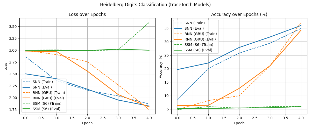
The current examples are limited to Spiking Heidelberg Digits (SHD) and MNIST. It was NOT optimized for SOTA performance or even good results to begin with. Rather, these are just examples to show how traceTorch layers integrate with PyTorch. As with PyTorch, the best results arise from clever thinking, not the library itself.
For example, running examples/heidelberg_digits/main.py will train an SNN (252k), RNN (973k), and SSM (227k) models,
and plot the following graph:
There is also examples/mnist/ with three different approaches:
rate_coded.py: Rate-coded SNN using Bernoulli sampling over 20 timestepssequential.py: Sequential processing by splitting images into patches and processing them as a sequencenoisy.py: Robustness testing with additive noise during training
Each example trains SNN, RNN, and SSM variants for comparison, demonstrating how traceTorch layers can handle different data modalities and processing strategies.
Authors
Contributing
Contributions are always welcome. Feel free to fork, submit pull requests or report issues, I will occasionally check in on it.
Roadmap
traceTorch is nearing its v1.0.0 release!
- Fix
tt.functionalto be cleaner - Clean up
tt.plotplotting functions Clean up and make sure that thesave_statesandload_stateswork as intended without faultCreate tests for compilation and decompilation, saving and loading- Finish the
examples/section for example code for various examples Make proper requirements for each example inexamples/- Write the documentation
- Make docstrings
Figure out versioning requirements for the library
Release history Release notifications | RSS feed


Download files
Download the file for your platform. If you're not sure which to choose, learn more about installing packages.
Source Distribution
Built Distribution
Filter files by name, interpreter, ABI, and platform.
If you're not sure about the file name format, learn more about wheel file names.
Copy a direct link to the current filters
File details
Details for the file tracetorch-0.19.1.tar.gz.
File metadata
- Download URL: tracetorch-0.19.1.tar.gz
- Upload date:
- Size: 36.3 kB
- Tags: Source
- Uploaded using Trusted Publishing? No
- Uploaded via: twine/6.2.0 CPython/3.13.13
File hashes
| Algorithm | Hash digest | |
|---|---|---|
| SHA256 |
a8eca4efcbf557d1af5dc854d201093c4b9c0ccfe66c284e266c2b257387dda3
|
|
| MD5 |
7624e91494d764895a109f03be53c57f
|
|
| BLAKE2b-256 |
540b36a5e334686eba88c5cef6d25b6a25e54f73e7f8a5a044b3f455ffe76002
|
File details
Details for the file tracetorch-0.19.1-py3-none-any.whl.
File metadata
- Download URL: tracetorch-0.19.1-py3-none-any.whl
- Upload date:
- Size: 40.3 kB
- Tags: Python 3
- Uploaded using Trusted Publishing? No
- Uploaded via: twine/6.2.0 CPython/3.13.13
File hashes
| Algorithm | Hash digest | |
|---|---|---|
| SHA256 |
3869b263f3ded010f6f107dab7ffe44609da2cdd1c25bc9f9155dbce00e0b6c4
|
|
| MD5 |
a2ab5e21589bc4d1b4205cf038481727
|
|
| BLAKE2b-256 |
4594583a0701cb7ebfb833043fee5467c994f4fe33adf7478c5c87b16e80067d
|


