
ttl3d






Turn any Turtle / RDF graph into a single self-contained HTML page with a 3D view (shaded spheres) and a 2D view (a flat canvas), permanent labels, predicate labels on the edges, a clickable legend, label search, and a detail card for every node. The page embeds all of its JavaScript, so it opens from a file, works offline, and never sends your data anywhere.
Try it in your browser: the Solar System demo (as two Turtle files, and as one TriG dataset with named graphs), FOAF, SKOS, PROV-O and the Pizza ontology, each a page ttl3d generated.
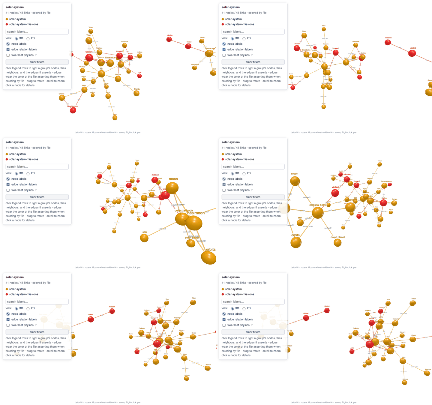
Why
Ontology editors show class trees. SPARQL browsers show one neighbourhood at a time. Sometimes you want the whole graph on screen at once: to see which modules actually connect, which file asserted which edge, or which node everything hangs from. ttl3d was written for exactly that while building a multi-file ontology, then generalized to any RDF input.
Install
Python 3.10 or newer.
pip install ttl3d
or, from conda-forge (Python 3.11 or newer there):
conda install -c conda-forge ttl3d
For the development version, pip install git+https://github.com/soheilabadifard/TTL_to_3D,
or clone the repository and run pip install -e .. The dependencies are
rdflib, networkx, numpy and scipy.
Quick start
ttl3d examples/solar-system.ttl examples/solar-system-missions.ttl -o solar.html
Open solar.html in any browser. Pass several files and they merge into one
graph; the default colouring then shows which file declared each node and
which file asserted each edge. A TriG or N-Quads file works the same way: each of its named
graphs is treated as a file of its own:
ttl3d examples/solar-system.trig -o solar-graphs.html
The same Solar System as one TriG dataset: the schema in the default graph, the bodies and the missions in two named graphs, one legend row each.
Without installing, run the module from a clone: python -m ttl3d ....
Python and notebooks

The same pipeline is a function call (pip install "ttl3d>=0.4.0"; tables and DataFrames need
ttl3d>=0.9.0). Sources are file paths, rdflib.Graph or rdflib.Dataset objects, ttl3d.Query
objects (a CONSTRUCT against a SPARQL endpoint), DataFrames (see "From tables"), (name, source)
pairs or a {name: source} mapping, in any mix, several in a list (not a set: their order names the
page and orders the legend); the options are the command line's (focus, hops, schema, columns
and base included).
import rdflib, ttl3d

g = rdflib.Graph().parse("solar-system.ttl")
ttl3d.write(["solar-system.ttl", "solar-system-missions.ttl"], "solar.html", view="2d")
html = ttl3d.to_html(("planets", g), color_by="type")        # the page as a string
ttl3d.show(("planets", g), height=500)                       # last line of a notebook cell: shown inline
show returns a page that Jupyter, JupyterLab, VS Code and Colab display as a sandboxed iframe
with the whole page inside, so nothing is written and no server is needed; each output stores
about 1.9 MB in the notebook. Errors are raised, never printed. examples/ttl3d.ipynb is the
notebook behind the badge.
Options
| Option | Values | Meaning |
|---|---|---|
- (as a file) |
Read standard input, parsed as --format (an rdflib format, or csv/tsv for a table) or Turtle; the page and the default output name are called stdin. Relative IRIs resolve against the working directory (a file's resolve against its folder); declare @base to be explicit. |
|
-o, --out |
path | Output file. Default: <first source's name>-<view>.html in the current directory (a file's stem, stdin, a query file's stem, or the endpoint's host for inline query text), with any colon as _: an IPv6 endpoint http://[::1]:8890/sparql writes __1-3d.html. |
--color-by |
file (default), type, namespace |
What node colours and the legend mean. In file mode edges also take the colour of the file asserting them. A named graph of a TriG or N-Quads file counts as a file. |
--layout |
auto (default), stress, force |
stress pins every node to a precomputed Kamada-Kawai position, one layout per view (3D and 2D); force runs the live simulation. auto picks stress up to 1000 nodes. |
--labels |
auto (default), always, hover |
Permanent label sprites. auto keeps node labels up to 800 nodes and edge labels up to 800 links; hover leaves tooltips only. |
--view |
3d (default), 2d |
Starting view. The page has a 3D | 2D switch either way, and each view is pinned to its own stress layout. |
--title |
text | Page title. Default: the first source's name (a file's stem, stdin, a query file's stem, or the endpoint's host for inline query text). |
--lang |
language tag, default en |
Preferred language for labels and definitions. Untagged literals rank next; other languages become synonyms on the card. Matched exactly: --lang en does not select @en-GB. |
--format |
rdflib parser name, csv, tsv |
Force a parser for every input (turtle, xml, nt, json-ld, trig, nquads, ...), or read every input as a table (csv, tsv). Default: guess from the extension, then try Turtle. |
--columns |
ROLE=HEADER[,...] |
The table column that plays a role when its header is not a known name: id, label, type, description, source, target or relation (see "From tables"). Repeatable; applies to every table of the run. |
--base |
IRI | The namespace for table ids that are neither IRIs nor CURIEs. Default urn:x-ttl3d:, shown as the prefix csv (csv2 when an input binds csv to another namespace). |
--type-links |
flag | Draw rdf:type as an edge from each instance to its class instead of listing it on the card only. |
--attribute-preds |
prefix:local, full IRI, or <urn:...> |
Predicates to keep off the picture and show on the card, e.g. foaf:homepage,rdfs:seeAlso. Repeatable; wrap a URN or mailto in angle brackets. |
--focus |
prefix:local, full IRI, or <urn:...> |
Keep only this node's neighbourhood (with --hops). Repeatable or comma-separated. |
--hops |
integer, default 1 | How many link steps from a focus node to keep; 0 keeps the focus nodes only. Needs --focus. |
--schema |
flag | Keep classes and properties only: the schema, without instances. |
--endpoint |
URL | A SPARQL endpoint (http or https) to run every --query against. Credentials come from TTL3D_SPARQL_USER and TTL3D_SPARQL_PASSWORD (HTTP Basic) or TTL3D_SPARQL_TOKEN (Bearer), never from the command line; a URL carrying user:password@ is refused. |
--query |
CONSTRUCT ... or @file.rq |
A CONSTRUCT or DESCRIBE query whose result is a source: a legend row named after the file, or after the endpoint's host for inline text. Repeatable. SELECT, ASK and updates are refused before anything is sent. |
--timeout |
seconds, default 60 | How long to wait for each network step (connect, read) of the endpoint's answer; one attempt, no retry. |
--max-mb |
megabytes, default 100 | The largest answer to accept; a bigger one is refused with a hint to narrow the query. Parsing needs about 35 times an N-Triples answer's size in memory, and more for Turtle. |
--version |
flag | Print ttl3d <version> and exit. |
Input formats are guessed from the extension (.ttl, .nt, .n3, .rdf,
.owl, .jsonld, .trig, .nq, ...) through rdflib; .csv and .tsv files are tables (see
"From tables"). A quad format (TriG,
N-Quads, TriX, JSON-LD with named @graph blocks) loads every named graph, and
each named graph is a source like a file: a legend row of its own, named by its
prefixed IRI (ex:planets, or the full IRI when no prefix covers it; the IRI
itself is the row's hover text and appears on the cards), while the file's
default graph keeps the file's name. The same graph IRI in several files is one
source.
What becomes a node, what becomes a link
- A node is every IRI that is the subject of some triple or the object of a
link, except IRIs of the RDF, RDFS, OWL and XSD vocabularies and ontology
headers (
owl:Ontology). Blank nodes are skipped. - A link is an IRI-to-IRI triple whose predicate is a relation.
rdf:type,owl:imports,owl:versionIRI,owl:priorVersion,rdfs:isDefinedBy,prov:wasDerivedFromanddcterms:sourcedescribe the node instead and go to its card. Parallel edges collapse into one link listing every predicate. - Label:
rdfs:label, elseskos:prefLabel, else the local name. Definition:skos:definition, elserdfs:comment, elsedcterms:description. Every other literal lands in the card's property table. - Each node remembers the file or named graph that first declares it, in the order sources and their graphs first appear; each link remembers the files or graphs asserting it. Every source has a legend row: a file that only adds edges between other files' nodes selects those edges, and a file that only annotates (labels, comments) gets a muted row that says so, since nothing it asserts is drawable.
- An edge asserted in both directions (
:Luna :orbits :Earthand:Earth :hasMoon :Luna) is one link labelledorbits ⇄ hasMoon, without an arrowhead. - Labels follow
--lang: the requested language first, then untagged literals, then anything else; every other label value becomes a synonym on the card, and ardfs:commentthat loses to askos:definitionstill appears in the property table. - Namespaces follow the prefixes the inputs bind: an IRI is cut at its last
/or#when that namespace is bound, otherwise at the longest bound namespace it extends without a further/or#(sourn:vocabularies shorten too), otherwise at the last/or#. Legend keys, the namespace column and local names all use this one rule. - A reified statement (
rdf:subject,rdf:predicate,rdf:object) about a drawn link puts its other properties on the card, under that relation: edge properties. Its triple must be asserted; a statement whose subject is an IRI is still a node as well. - Types, edge labels and property names are local names, unless two of those the page shows
share one: then both show their prefix (FOAF types its classes
owl:Classandrdfs:Class;dc:titleanddcterms:title), or the full IRI when their namespace has no prefix.
Slicing a big graph
A knowledge graph of a million triples is not a picture. Two questions are, and both are answered at build time, before the layout runs:
ttl3d examples/solar-system.ttl examples/solar-system-missions.ttl --focus :Earth --hops 2 -o earth.html
ttl3d examples/solar-system.ttl examples/solar-system-missions.ttl --schema -o schema.html
--focus keeps a node and everything within --hops link steps of it, in both directions;
rdf:type and the other card-only predicates are not steps unless --type-links makes them
edges, and with --type-links every kept node's classes come along so no card loses its type.
--schema keeps the classes and properties (anything typed as one, used as a type, or joined by
rdfs:subClassOf, rdfs:subPropertyOf, rdfs:domain, rdfs:range, and the OWL equivalence,
inverse and disjointness predicates) and drops every instance; with --focus as well, the walk
stays inside the schema, and a focus that is itself an instance is kept. A kept node keeps its
labels, literals, blank-node structure and card-only attributes (a dcterms:source target outside
the slice shows as an IRI); an edge survives only when both ends do; a source left with nothing
loses its legend row, and a node's source is the first source that still says something about it
in the slice. ttl3d says what it kept on stderr: kept 12 of 41 nodes (focus :Earth, 2 hops).
The same three keyword arguments exist on ttl3d.to_html, write and show.
Slicing does not skip the parse: rdflib reads about a million triples in 13 seconds and 2.3 GB (measured on a 200-class, 200,000-instance file), after which a two-hop slice builds in under 1.5 seconds and a schema slice in under 1.5 seconds. The cost of a slice follows the triples that survive, not the nodes: one subject with 200,000 literal attributes took 4 seconds at hop 0.
From a SPARQL endpoint
A triple store is drawn without exporting it: a CONSTRUCT (or DESCRIBE) query is a source like a file, fetched at build time with one POST and never from the page.
ttl3d --endpoint https://query.wikidata.org/sparql --query @examples/wikidata-moons.rq -o moons.html
# fetched 916 triples from query.wikidata.org in 0.7 s
# computing stress layouts (3D and 2D) for 308 nodes...
# 308 nodes, 300 links -> moons.html (view: 3d, layout: stress, labels: node+edge)
--query repeats, each result its own legend row, and files and queries mix in one page. The query's
PREFIX lines name the page's namespaces, so an endpoint that answers in N-Triples still gets short
names; relative IRIs in an answer resolve against the endpoint. Protected endpoints take
TTL3D_SPARQL_USER/TTL3D_SPARQL_PASSWORD or TTL3D_SPARQL_TOKEN from the environment, and nothing
ttl3d prints shows them. ttl3d sends them to whatever endpoint the command names, so set them for one
command (TTL3D_SPARQL_TOKEN=... ttl3d ...) rather than exporting them; the fetch line on stderr says
when credentials went out, and when they went over plain http. Errors are one line, and name the
endpoint's port when its URL gives one: a query that is not CONSTRUCT or DESCRIBE is refused before
anything is sent, an HTTP error quotes the endpoint's first line, a slow endpoint stops at --timeout
(60 s per network step by default), a redirect is refused with the URL to use, and an answer that is not RDF (Turtle, N-Triples, RDF/XML, N3 or a quad format;
JSON-LD is refused too), is larger than --max-mb (100 MB) or breaks off midway is refused rather than
drawn in part. RDF/XML and TriX, from an endpoint or a file, pass through Python's expat parser before
rdflib reads them: entities that nest into gigabytes ("billion laughs") are refused in milliseconds,
and external entities are never fetched. In Python the same source is ttl3d.Query:
import ttl3d

query = open("examples/wikidata-moons.rq", encoding="utf-8").read()
moons = ttl3d.Query("https://query.wikidata.org/sparql", query)
ttl3d.write(("moons", moons), "moons.html", color_by="type")
ttl3d.show(["examples/solar-system.ttl", ("moons", moons)], focus=["wd:Q2"], hops=1)   # Earth and its moons, sliced
A namespace is named by the first source that binds it, so list a file first when you focus with its
prefixes. The answer parses like a file (about 13 s and 2.3 GB per million triples), so let the query
select the piece: a VALUES list or a LIMIT keeps an answer small, and --focus/--schema trim
further.
From tables (CSV, TSV, DataFrames)
A property graph exported from Neo4j, Gephi or networkx, or a hand-made spreadsheet, is drawn as it is: an edge table, and a node table if there is one. No mapping file: the header says what each column is.
ttl3d examples/missions.csv examples/mission-links.csv --color-by type -o missions.html
# 28 nodes, 35 links -> missions.html (view: 3d, layout: stress, labels: node+edge)
A .csv or .tsv file is a table; --format csv (or tsv) reads any file, and standard input
(-), as one. A table with source and target columns is an edge table, one with an id column a node
table, and every other column is a property. Headers are matched in any case; when a table has several
headers for one role, the first listed here wins and the others are properties:
| Role | Headers |
|---|---|
| id | id, node, key, :ID, _id |
| label | label, name, title |
| type | type, types, class, category, kind, :LABEL, _labels, labels (several types split on ;, APOC's _labels on : as in :Person:Actor) |
| description | description, definition, comment (the card's definition) |
| source | source, src, from, start, subject, head, :START_ID, _start |
| target | target, dst, to, end, object, tail, :END_ID, _end |
| relation | relation, predicate, rel, :TYPE, _type, label, type |
Neo4j's import headers work as written (personId:ID(Person), :START_ID(Person), born:int,
roles:string[] split on ;, :IGNORE; the kinds in capitals, as Neo4j writes them, so a header
such as rdfs:label or dc:type keeps its RDF meaning). The data types (born:int,
roles:string[]) are read in a table that has an :ID, :START_ID or :END_ID column, so RDF
headers such as dc:date keep their meaning. Ids in different ID groups stay different
nodes, and APOC's one-file export (nodes and relationships in one table) works too. Gephi's edge
Label is the relation and its Type (Directed/Undirected) an edge property. Any other header is
mapped by hand, for every table of the run: --columns source=from_id,target=to_id
(columns={"source": "from_id"} in Python); a column you map is not also taken by another role's
names. The delimiter of a .csv (comma, semicolon or tab) is read from the header line; the text must
be UTF-8, and a quote left open is an error naming its line rather than a cell that swallows the rest
of the file.
- Ids.
<urn:isbn:0441013597>, or anything with://, is that IRI.ex:Duneis a CURIE when an RDF file of the same run bindsex, so a table can add edges between an ontology's nodes;Person:1stays a plain id when no file bindsPerson. rdflib binds its well-known prefixes (schema,foaf,dc,dcterms,org,time, ...) on every RDF file it reads, so with an RDF file in the run those CURIEs resolve too; in a table-only run they are plain ids. Any other id becomesurn:x-ttl3d:<id>(--basepicks another namespace), shown with the prefixcsv(csv2when an input already usescsvfor something else):--focus csv:voyager2. A minted id is percent-encoded, so--focusnames an id with a space ascsv:New%20York(the card's IRI shows the form to use). Every table of a run shares these ids, so a node table and an edge table meet, and a node keeps its id as its label unless a node table names it. - Edges. An edge row draws
source relation target; without a relation the edge isrelated. Relations, types and property names follow the id rules, with spaces as_(operated byreadsoperated_by). - Edge properties. The other cells of an edge row show on the card of both ends, under the
relation row:
kind flyby · year 1979, followed by the sources that hold them when the page has several, as relation rows do. They are stored the RDF way, as a reified statement (rdf:Statement), and an RDF file that reifies its edges gets the same lines on its cards.
In Python a DataFrame is a table too. ttl3d reads it through to_csv, so pandas is never imported
and never required; a named index (set_index("id")) counts as a column. Read the files as text
(dtype=str), or pandas turns a year with gaps into 1969.0:
import pandas as pd, ttl3d

missions = pd.read_csv("examples/missions.csv", dtype=str)
links = pd.read_csv("examples/mission-links.csv", dtype=str)
ttl3d.show([("missions", missions), ("mission-links", links)], color_by="type")
Measured on 100,000 edge rows between 20,000 nodes: 1.3 s to load and 1.7 s to build without
property columns (0.5 GB), 7.0 s and 4.6 s with two of them (1.6 GB), since every row with properties
becomes a reified statement. A graph that size is far past the stress layout's reach: slice it with
--focus.
In the page
- Legend rows filter inclusively: a selected group keeps its own nodes, their direct neighbours, and the endpoints of every edge it asserts, whether or not another source asserted that edge first.
- The
3D | 2Dswitch rebuilds the picture in the other view. Legend filters, the search text and the open card carry over, and in pinned mode each view has its own precomputed stress layout. A browser without WebGL opens in 2D and says so. - Search dims everything whose label does not match.
- The keyboard works too: Tab reaches the legend rows (Enter or Space toggles one), Enter in the search box opens the card of the best match (the exact label, then labels starting with the text), Tab and Enter walk the card's relations to the neighbours' cards, and Esc closes the card. Legend rows, relations and the close button are labelled for screen readers.
- Click a node for its card: types, source (the file, or the named graph with its IRI), namespace, definition, synonyms, properties, incoming and outgoing relations (clickable), and sources.
- The label toggles rebuild the scene, so a big graph can start without sprites and switch them on later.
- "Free-float physics" releases pinned nodes into the live force layout and pins them back where they were.
- No fog: white fog made distant nodes vanish on zoom-out.
- Past twelve groups only the eleven largest keep a colour; the rest share one grey "other" row that filters them together.
Scale
The stress layout is quadratic in the number of nodes and label sprites are scene objects, so the automatic modes degrade instead of freezing:
| Graph size | Layout | Labels |
|---|---|---|
| up to 800 nodes / 800 links | pinned stress layout | nodes and edges |
| up to 1000 nodes | pinned stress layout | tooltips for the layer over its threshold |
| larger | live force simulation | tooltips; switch sprites on from the panel |
For inputs far beyond these sizes, slice them first: see "Slicing a big graph". A store behind a SPARQL endpoint answers with the piece you ask for: see "From a SPARQL endpoint".
The stress layout is computed twice, once per view, so a pinned page takes about twice the layout time of 0.1.0.
Force the behaviour you want with --layout and --labels.
Limitations
- Blank nodes are skipped, so OWL restrictions and RDF lists do not appear.
- No reasoning: only asserted triples are drawn.
- One page holds one graph; there is no incremental loading.
- The stress layout is quadratic:
--layout stresson graphs far beyond 1000 nodes can take minutes, and the CLI says so on stderr.
Development
pip install -e .[test]
python -m pytest -q
The tests cover the loader, the node and link rules, the layout, the generated page, the vendored
bundle's pins and licence notices, and the command line. The viewer's CSS and JavaScript live in ttl3d/viewer.css, ttl3d/viewer.js (shared by both views), ttl3d/viewer-3d.js and ttl3d/viewer-2d.js (one renderer per view)
and are inlined into every page; when node is installed the suite syntax-checks the
JavaScript. pip install -e .[browser] && playwright install chromium enables the headless
browser tests that load the demo pages, switch views and assert zero console errors
(TTL3D_BROWSER=firefox or webkit picks another engine). CI runs the suite on Linux, Windows
and macOS, the browser tests on Chromium, Firefox and WebKit, and checks that the demo pages
built on the three systems are identical apart from the pinned layout's last digits. The vendored JavaScript
in ttl3d/vendor/ bundles 3d-force-graph, force-graph, three-spritetext and one shared three.js;
VENDOR.md there has the rebuild recipe and LICENSES.md the upstream notices.
Citing
If ttl3d helped your work, cite it: CITATION.cff holds the reference and GitHub's "Cite this
repository" button renders it as BibTeX or APA. Every release is archived on Zenodo; the DOI
10.5281/zenodo.22716060 always resolves to the latest one.
License
MIT. The vendored JavaScript is under permissive licences (MIT, ISC and others); ttl3d/vendor/LICENSES.md lists every bundled package with its licence and copyright line.
1 maintainer

Metadata
1 maintainer
Release files for ttl3d 0.9.0
For a detailed explanation of source distributions (sdists) and built distributions (wheels), please see the package formats documentation.
Source distribution (sdist)
| File | Size | Uploaded | |
|---|---|---|---|
| ttl3d-0.9.0.tar.gz | 586.4 kB | Details |
Built distribution (wheel)
| File | Interpreter | ABI | Platform | Reset |
|---|---|---|---|---|
| ttl3d-0.9.0-py3-none-any.whl | Python 3 | none | any | Details |
Total release size: 1.1 MB
Release files / ttl3d-0.9.0.tar.gz
| Download URL | ttl3d-0.9.0.tar.gz |
|---|---|
| Size | 586.4 kB |
| Tags | Source |
|
SHA-256 checksum How to use checksums |
bf3fc9a97550066e100c3409f101803ceebf75a7455615ac12e702db4417d584
|
|
BLAKE2b-256 checksum How to use checksums |
2cb863e67138a0d89c0d7a8aad189668e644286715b153e47acdd8d6693c1ce3
|
| Upload date | |
|
Uploaded using Trusted Publishing? What is trusted publishing? |
Yes |
| Uploaded via |
twine/7.0.0 CPython/3.13.14
|
Provenance
Provenance describes where a file came from. On PyPI, provenance is shared via attestations, which provide a verifiable record of the build or publishing details. View details, limitations and caveats.


PyPI Publish Attestation
PyPI verified that this artifact, at this checksum, originated from the publisher listed below.
Signed by GitHub Actions, verified by PyPI on Oct 15, 2026.
Transparency logRelease files / ttl3d-0.9.0-py3-none-any.whl
| Download URL | ttl3d-0.9.0-py3-none-any.whl |
|---|---|
| Size | 528.5 kB |
| Tags | Python 3 |
|
SHA-256 checksum How to use checksums |
68330482085855a6665363e81af7cd1fd45d9bab112ce4404f9b531c5a17b4bc
|
|
BLAKE2b-256 checksum How to use checksums |
efdf120f24e3b05b3d537a26021c2dd5f0062c79c5285a2386d68d8050d1b49a
|
| Upload date | |
|
Uploaded using Trusted Publishing? What is trusted publishing? |
Yes |
| Uploaded via |
twine/7.0.0 CPython/3.13.14
|
Provenance
Provenance describes where a file came from. On PyPI, provenance is shared via attestations, which provide a verifiable record of the build or publishing details. View details, limitations and caveats.
PyPI Publish Attestation
PyPI verified that this artifact, at this checksum, originated from the publisher listed below.
Signed by GitHub Actions, verified by PyPI on Oct 15, 2026.
Transparency log













