Time-Varying Coefficient regression and Generalized Cointegration (Hall, Swamy & Tavlas)

Project description
tvccointreg
Time-Varying-Coefficient regression and Generalized Cointegration in Python.
tvccointreg implements the generalized cointegration framework of
Hall, S. G., Swamy, P. A. V. B., & Tavlas, G. S. (2015). A Note on Generalizing the Concept of Cointegration.
together with the surrounding Swamy time-varying-coefficient (TVC) literature (Swamy & Mehta 1975; Swamy, Tavlas, Hall & co-authors 2003–2014; Granger 2008).
Conventional cointegration (Engle–Granger 1987) is an inherently linear
concept: it can only recover a structural relationship if that relationship
happens to be linear in unit-root variables. Most economic theory, however,
implies nonlinear relationships among variables that are nonstationary but
not necessarily unit-root. tvccointreg lets you:
- estimate a model that is linear in variables but with time-varying coefficients — the Swamy–Mehta / Granger representation of any nonlinear relationship (eq. 7);
- decompose each coefficient into a bias-free structural component plus omitted-variable bias and measurement-error bias using coefficient drivers (eq. 8);
- test for generalized cointegration — i.e. whether the bias-free structural partial derivative is nonzero — with standard χ²/normal inference (no Dickey–Fuller tables);
- produce journal-quality tables (text / LaTeX booktabs / HTML) and publication-quality plots with the MATLAB Parula colormap by default.
Table of contents
- Installation
- The 60-second tour
- Concepts: how the paper maps to the code
- The estimator
- API reference
- Detailed syntax
- Visualizations
- Worked example: spurious vs. real
- Testing
- Citing
- References
Installation
# from a clone of the repo
git clone https://github.com/merwanroudane/tvccointreg.git
cd tvccointreg
pip install -e .

# with the optional ADF / test extras
pip install -e ".[dev]"
Requirements: numpy, scipy, pandas, matplotlib. statsmodels is optional
(used only for the ADF stationarity diagnostic and some examples).
The 60-second tour
from tvccointreg import TVCModel, DriverSpec
from tvccointreg.datasets import simulate_nonlinear_cointegration

# 1) A nonlinear relationship between nonstationary variables.
sim = simulate_nonlinear_cointegration(T=300, seed=1, nonlinearity=0.4)

# 2) Partition the drivers into the three sets (Assumption 1 / eq. 8).
spec = DriverSpec(
    names=list(sim.drivers.columns),
    bias_free=["x_lag", "y_lag"],   # true coefficient variation
    omitted=["w"],                  # omitted-variable bias
    measurement=[],                 # measurement-error bias
)

# 3) Fit by iteratively rescaled GLS.
res = TVCModel(sim.y, sim.X, sim.drivers, driver_spec=spec).fit()

# 4) Journal table + generalized cointegration test.
print(res.summary())
res.coint_test()
==============================================================================
      Time-Varying-Coefficient Regression  /  Generalized Cointegration
==============================================================================
Dep. variable: y                       No. observations: 300
No. coefficients: 2                    No. drivers: 3
Estimator: Iteratively rescaled GLS    Covariance: GLS
R-squared: 0.8311                      Log-likelihood: -78.07
Converged: True                        Resid ADF p-value: 0.0000
==============================================================================
Variable    Coef (mean)  Bias-free    Std.Err          t    p-value    G-Coint
------------------------------------------------------------------------------
x                0.3283     0.3392     0.0698     4.8614     0.0000 ***     Yes
==============================================================================
                   Signif.: *** p<0.01  ** p<0.05  * p<0.10
       Bias-free = structural derivative; G-Coint via Wald test on it.
==============================================================================
On this DGP the recovered bias-free coefficient correlates 0.99 with the true time-varying derivative, and the residuals are stationary (ADF p ≈ 0) — exactly the standard-inference result the paper proves.
Concepts: how the paper maps to the code
| Paper (Hall–Swamy–Tavlas 2015) | Symbol | In tvccointreg |
|---|---|---|
| TVC model, eq. (7) | y_t = γ_0t + γ_1t x_1t + … + γ_{K-1,t} x_{K-1,t} |
TVCModel(y, X, drivers) |
| Coefficient-driver eq., eq. (8) | γ_jt = π_j0 + Σ_d π_jd z_dt + ε_jt |
DriverSpec(...) + the drivers matrix |
| Three components of a coefficient | bias-free / omitted-variable / measurement-error | DriverSpec(bias_free=, omitted=, measurement=) |
| Concentrated model | y_t = w_t'π + u_t, u_t = Σ_j x_jt ε_jt |
estimation.build_design, estimation.irgls |
| Variance structure | Var(u_t) = Σ_j σ_j² x_jt² |
estimation.variance_components (Hildreth–Houck–Swamy) |
| Consistent estimator (§3.3) | iteratively rescaled GLS | TVCModel.fit(method="irgls") |
| Bias-free component | γ_jt^BF = π_j0 + Σ_{d∈BF} π_jd z_dt |
res.bias_free_coefficients() |
| Generalized cointegration, eqs. (5)–(6) | ∂y/∂x ≠ 0 ⇔ bias-free component ≠ 0 |
res.coint_test() |
| Standard inference (§3.3) | χ² Wald / normal, not Dickey–Fuller | Wald + delta-method t in cointegration.py |
| Drivers vs. instruments (Table 1) | drivers should be correlated with the misspecification | the omitted / measurement sets |
The definition, in one line
y and x are generalized-cointegrated if, holding all other relevant preexisting conditions w constant, the bias-free part of
∂y/∂xis nonzero.
Cointegration is thus a property of the real-world structural relationship, not of any particular statistical model — and it survives nonlinearity and omitted regressors.
The estimator
Substituting the driver equation (8) into the TVC model (7) gives a model that
is linear in the stacked parameter vector π:
y_t = w_t' π + u_t ,   w_t = ( x_0t·z_t , x_1t·z_t , … ) ,   u_t = Σ_j x_jt ε_jt
Var(u_t | x_t) = Σ_j σ_j² x_jt²          (Hildreth–Houck–Swamy structure)
tvccointreg then:
- OLS start on the concentrated design
W. - Variance components
σ_j²from a non-negative regression of squared residuals on squared regressors (scipy.optimize.nnls). - GLS with weights
1/h_t,h_t = Σ_j σ_j² x_jt²; iterate to convergence (iteratively rescaled GLS). - Recover the time-varying coefficients
γ_jt = z_t'π_j + ε̂_jt, where the random part is the best linear predictorε̂_jt = σ_j² x_jt u_t / h_t. - Decompose
γ_jtinto bias-free / omitted / measurement parts using the driver-set masks, and test the bias-free block.
Inference uses the GLS covariance (W'Ω⁻¹W)⁻¹ (the paper's standard-inference
result) or a heteroskedasticity-robust sandwich (cov_type="robust").
Note / honest caveat. As in the paper, validity hinges on Assumption 1 — that the chosen drivers genuinely span the bias components. This is an identifying assumption, not something the data can confirm; choose drivers that are plausibly correlated with the suspected misspecification (Table 1).
API reference
TVCModel(y, X, drivers, driver_spec=None, driver_sets=None, add_const=True, index=None)
Build a model. y (T,), X (T, K−1), drivers (T, m). A constant regressor and
a constant driver are added automatically. Accepts NumPy arrays or pandas
objects (column names are picked up automatically).
.fit(method="irgls", max_iter=100, tol=1e-8, cov_type="gls", verbose=False)→TVCResults.
DriverSpec(names, bias_free=[], omitted=[], measurement=[])
Three-set partition of the drivers. Any driver not listed defaults to
bias_free. .describe() prints the partition.
TVCResults
| Method | Returns |
|---|---|
| `.summary(fmt="text" | "latex" |
.coef_table() |
per-regressor average coefficient frame |
.coint_test(alpha=0.05, skip_const=True) |
tidy DataFrame of test results (and .coint_results_) |
.tv_coefficients(include_random=True) |
T×K time-varying coefficients |
.bias_free_coefficients() |
T×K bias-free (structural) coefficients |
.components(regressor) |
bias-free / omitted / measurement / random / total |
.coefficient_se() |
pointwise standard errors |
.diagnostics() |
R², log-lik, convergence, residual ADF |
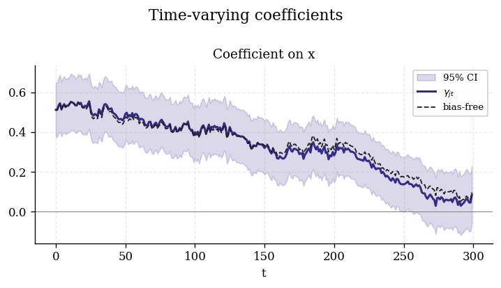
.plot_coefficients(...) |
TVC paths with CI bands |
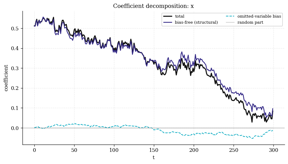
.plot_decomposition(regressor) |
the three-component decomposition |
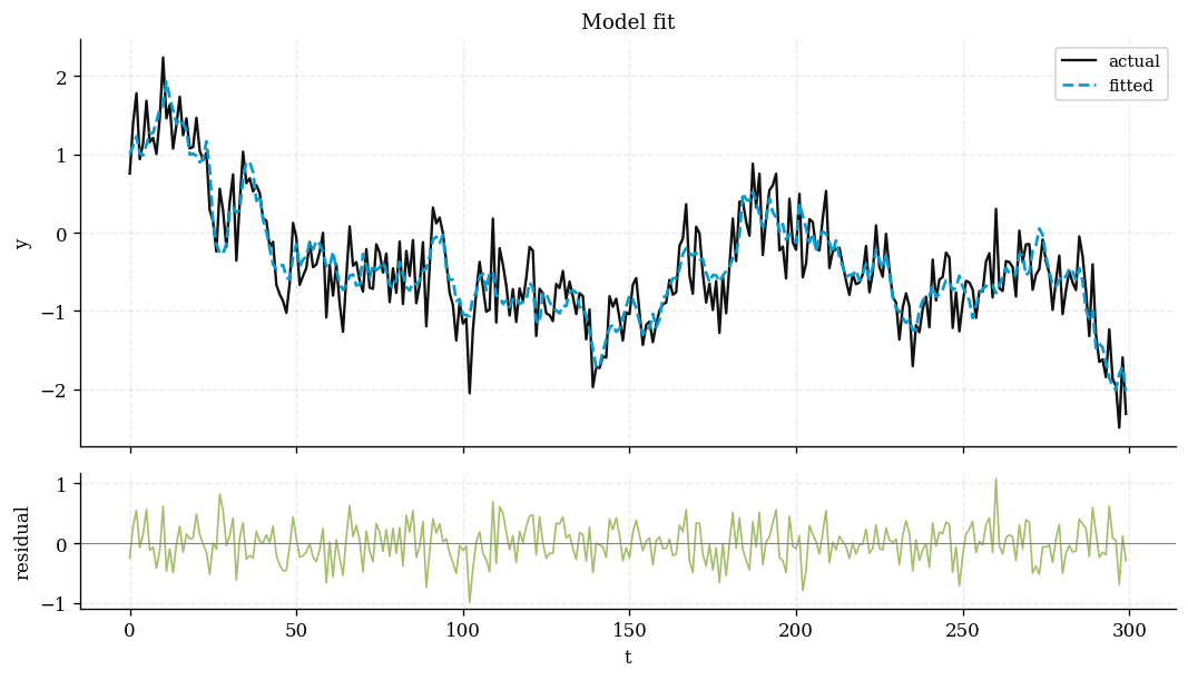
.plot_fit() |
actual vs fitted + residuals |
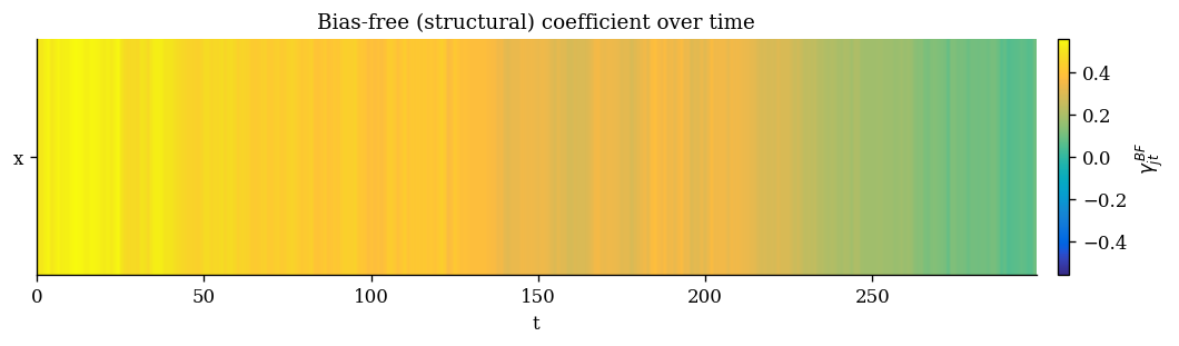
.plot_coint_heatmap() |
Parula heatmap of bias-free paths |
Datasets
simulate_nonlinear_cointegration(T, seed, nonlinearity, omitted, measurement_error)simulate_spurious(T, seed)
Colormaps
parula_colors(n), matlab_jet_colors(n), turbo_colors(n), bluered_colors(n),
sinha_colors(n), resolve_colorscale("Parula", n), get_cmap("parula").
Detailed syntax
Using raw NumPy arrays and reading off a specific test:
import numpy as np
from tvccointreg import TVCModel, DriverSpec

res = TVCModel(y, X, Z,                       # y:(T,), X:(T,K-1), Z:(T,m)
               driver_sets={"bias_free": ["z1"],
                            "omitted":   ["z2"],
                            "measurement": ["z3"]}).fit()

ct = res.coint_test()
print(ct.loc["x1", "cointegrated"], ct.loc["x1", "p_value"])
Robust covariance and OLS (homoskedastic) comparison:
res_robust = TVCModel(y, X, Z, driver_spec=spec).fit(cov_type="robust")
res_ols    = TVCModel(y, X, Z, driver_spec=spec).fit(method="ols")
Exporting a LaTeX table for a paper:
with open("table1.tex", "w") as f:
    f.write(res.summary(fmt="latex"))
Pulling the time-varying coefficient path of one regressor:
gamma_x = res.tv_coefficients()["x"]          # pandas Series indexed by t
bf_x    = res.bias_free_coefficients()["x"]
Visualizations
All plots default to the MATLAB Parula colormap and return a matplotlib
Figure.
plot_coefficients() |
plot_decomposition("x") |
 |
 |
plot_fit() |
plot_coint_heatmap() |
 |
 |
Worked example: spurious vs. real
examples/spurious_vs_real.py reproduces the central point of the paper:
================ SPURIOUS (independent random walks) ================
Naive OLS slope = 1.125  (p = 5.97e-46)   <- spuriously 'significant'
Generalized cointegration: NO (p = 0.708)

================ GENUINE generalized cointegration ================
Generalized cointegration: YES (p = 1.34e-35)
A naive OLS regression of one random walk on another is wildly "significant", yet the generalized-cointegration test on the bias-free component correctly finds no structural relationship.
Empirical application: the US consumption function (real data)
examples/real_data_consumption.py applies the method to real US quarterly
macro data (statsmodels macrodata, 1959Q1–2009Q3, 202 obs after lagging).
We model the long-run relationship between real personal consumption and
real disposable income (both in logs, both strongly trending / I(1)):
import numpy as np, pandas as pd
from statsmodels.datasets import macrodata
from tvccointreg import TVCModel, DriverSpec

d = macrodata.load_pandas().data
d.index = pd.period_range("1959Q1", periods=len(d), freq="Q")
zscore = lambda s: (s - s.mean()) / s.std(ddof=0)

y = np.log(d["realcons"]).rename("log_cons")
X = np.log(d[["realdpi"]]).rename(columns={"realdpi": "log_inc"})
drivers = pd.DataFrame({
    "inc_lag":  zscore(np.log(d["realdpi"]).shift(1)),
    "trend":    zscore(pd.Series(np.arange(len(d)), index=d.index)),
    "realint":  zscore(d["realint"]),
    "unemp":    zscore(d["unemp"]),
    "cons_lag": zscore(np.log(d["realcons"]).shift(1)),
})
df = pd.concat([y, X, drivers], axis=1).dropna()

spec = DriverSpec(
    names=["inc_lag", "trend", "realint", "unemp", "cons_lag"],
    bias_free=["inc_lag", "trend"],   # true elasticity variation
    omitted=["realint", "unemp"],     # interest-rate / labour-market channels
    measurement=["cons_lag"],         # dynamics / measurement
)
res = TVCModel(df["log_cons"], df[["log_inc"]], df[spec.names],
               driver_spec=spec, index=df.index.astype(str)).fit()
print(res.summary())
print(res.coint_test())
Result (verbatim output):
==============================================================================
Time-Varying-Coefficient Regression / Generalized Cointegration
==============================================================================
Dep. variable: log_cons No. observations: 202
No. coefficients: 2 No. drivers: 5
Estimator: Iteratively rescaled GLS Covariance: GLS
R-squared: 0.9999 Log-likelihood: 752.32
Converged: True Resid ADF p-value: 0.0000
==============================================================================
Variable Coef (mean) Bias-free Std.Err t p-value G-Coint
------------------------------------------------------------------------------
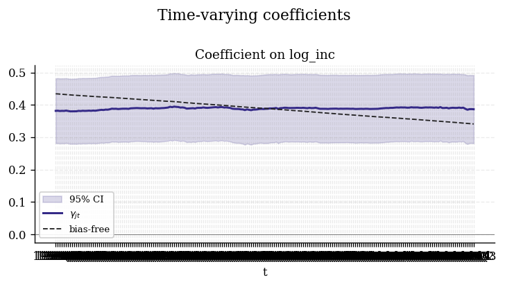
log_inc 0.3886 0.3886 0.0528 7.3626 0.0000 *** Yes
==============================================================================
| regressor | avg_bias_free | std_err | t_stat | wald | df | p_value | cointegrated |
|---|---|---|---|---|---|---|---|
| log_inc | 0.3886 | 0.0528 | 7.3626 | 56.9504 | 3 | 0.0000 | True |
Reading the result.
- Generalized cointegration is confirmed between consumption and income (Wald = 56.95, 3 df, p ≈ 0): the bias-free structural elasticity is firmly nonzero, so the long-run relationship is genuine, not spurious.
- Standard inference is valid here: the composite residuals are stationary (ADF p = 1.9 × 10⁻⁷), exactly the condition under which Hall–Swamy–Tavlas show the TVC test uses ordinary χ²/normal critical values rather than Dickey–Fuller ones.
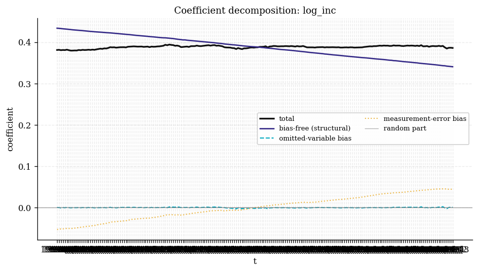
- The bias-free income elasticity drifts down over the sample, from 0.43
(1959Q2) to 0.34 (2009Q3) — the direct income channel after the
dynamics (
cons_lag) and omitted business-cycle conditions (realint,unemp) are stripped out into the bias terms. A declining direct sensitivity of consumption to current income over five decades is consistent with greater consumption smoothing / financial deepening.
| Bias-free income elasticity over time | Coefficient decomposition |
|---|---|
 |
 |
Run it yourself:
python examples/real_data_consumption.py
Testing
pip install -e ".[dev]"
pytest -q
The suite checks coefficient recovery, that the three components sum exactly to the total coefficient, detection of genuine generalized cointegration, rejection of spurious relationships, and the Parula palette/colorscale helpers.
Publishing (maintainer notes)
The package is PyPI-ready (python -m build + twine check both pass).
First release — manual upload with an API token
- Create accounts on TestPyPI and PyPI, and generate an API token for each (Account settings → API tokens).
- Build and check:
python -m build
python -m twine check dist/*
- Dry-run on TestPyPI first, then install from there to confirm:
python -m twine upload --repository testpypi dist/*
pip install --index-url https://test.pypi.org/simple/ \
    --extra-index-url https://pypi.org/simple/ tvccointreg
- Upload to the real PyPI:
python -m twine upload dist/*
When prompted, use__token__as the username and the API token (starting withpypi-) as the password.
Subsequent releases — automated via Trusted Publishing (recommended)
.github/workflows/publish.yml publishes automatically when you publish a
GitHub Release. One-time setup: on PyPI add a Trusted Publisher
(Project → Publishing) for repository merwanroudane/tvccointreg, workflow
publish.yml, environment pypi. After that, no tokens or secrets are needed —
just bump version in pyproject.toml and __version__, tag, and publish a
Release.
Remember: a version number can only be uploaded to PyPI once. Bump the version for every release.
Citing
If you use this package, please cite both the package and the underlying paper.
@software{roudane_tvccointreg,
  author  = {Merwan Roudane},
  title   = {tvccointreg: Time-Varying-Coefficient Regression and
             Generalized Cointegration in Python},
  year    = {2026},
  url     = {https://github.com/merwanroudane/tvccointreg}
}

@incollection{hall_swamy_tavlas_2015,
  author  = {Hall, Stephen G. and Swamy, P. A. V. B. and Tavlas, George S.},
  title   = {A Note on Generalizing the Concept of Cointegration},
  year    = {2015}
}
References
- Hall, S. G., Swamy, P. A. V. B., & Tavlas, G. S. (2015). A Note on Generalizing the Concept of Cointegration.
- Hall, S. G., Swamy, P. A. V. B., & Tavlas, G. S. (2014). Time Varying Coefficient Models; A Proposal for Selecting the Coefficient Driver Sets. University of Leicester WP 14/18.
- Swamy, P. A. V. B., & Mehta, J. S. (1975). Bayesian and non-Bayesian Analysis of Switching Regressions and of Random Coefficient Regression Models. JASA.
- Swamy, P. A. V. B., Tavlas, G. S., Hall, S. G., et al. (2010). Nonparametric Nonstationary Regression.
- Granger, C. W. J. (2008). Non-linear Models: Where Do We Go Next — Time-Varying Parameter Models? Studies in Nonlinear Dynamics & Econometrics.
- Hildreth, C., & Houck, J. P. (1968). Some Estimators for a Linear Model with Random Coefficients. JASA.
- Engle, R. F., & Granger, C. W. J. (1987). Co-integration and Error Correction. Econometrica.
- Cramér, H. (1946). Mathematical Methods of Statistics.
Author
Dr Merwan Roudane · merwanroudane920@gmail.com · github.com/merwanroudane
Released under the MIT License.
Release history Release notifications | RSS feed


Download files
Download the file for your platform. If you're not sure which to choose, learn more about installing packages.
Source Distribution
Built Distribution
Filter files by name, interpreter, ABI, and platform.
If you're not sure about the file name format, learn more about wheel file names.
Copy a direct link to the current filters
File details
Details for the file tvccointreg-0.1.0.tar.gz.
File metadata
- Download URL: tvccointreg-0.1.0.tar.gz
- Upload date:
- Size: 36.5 kB
- Tags: Source
- Uploaded using Trusted Publishing? No
- Uploaded via: twine/6.2.0 CPython/3.11.0
File hashes
| Algorithm | Hash digest | |
|---|---|---|
| SHA256 |
85adb4e862443f6517a63983abfe1a914b9fcfd26e2020ce3c1d30bee70ed4d6
|
|
| MD5 |
0e24a62abd3ac8c77f6307a626e9a0de
|
|
| BLAKE2b-256 |
794fb9f07aedeead92ebb97e4c8f78053fae82d669bfbf8123d25e1a77c3f24f
|
File details
Details for the file tvccointreg-0.1.0-py3-none-any.whl.
File metadata
- Download URL: tvccointreg-0.1.0-py3-none-any.whl
- Upload date:
- Size: 29.9 kB
- Tags: Python 3
- Uploaded using Trusted Publishing? No
- Uploaded via: twine/6.2.0 CPython/3.11.0
File hashes
| Algorithm | Hash digest | |
|---|---|---|
| SHA256 |
6ae3b6f7919e775057ed521a170797b0a42856fb164aba02fcd95f1b63fe7ae6
|
|
| MD5 |
88ac0f548ccb5dbb9ad287dcc07897e6
|
|
| BLAKE2b-256 |
6ab493e7d2127ba7bf95ad6077cc5f60fced5bca242eaaf846e7f5f40a3b6a58
|


