shap · PyPI

A unified approach to explain the output of any machine learning model.

These details have not been verified by PyPI

Project links

Project description

License Tests Downloads

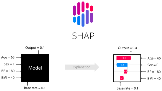
SHAP (SHapley Additive exPlanations) is a game theoretic approach to explain the output of any machine learning model. It connects optimal credit allocation with local explanations using the classic Shapley values from game theory and their related extensions (see papers for details and citations).

Install

SHAP can be installed from either PyPI or conda-forge:

pip install shap
or
conda install -c conda-forge shap

Contributing

We welcome contributions highly. Feel free to file an issue. Before opening a PR make sure you've read our CONTRIBUTING.md guideline.

Tree ensemble example (XGBoost/LightGBM/CatBoost/scikit-learn/pyspark models)

While SHAP can explain the output of any machine learning model, we have developed a high-speed exact algorithm for tree ensemble methods (see our Nature MI paper). Fast C++ implementations are supported for XGBoost, LightGBM, CatBoost, scikit-learn and pyspark tree models:

import xgboost
import shap

# train an XGBoost model
X, y = shap.datasets.california()
model = xgboost.XGBRegressor().fit(X, y)

# explain the model's predictions using SHAP
# (same syntax works for LightGBM, CatBoost, scikit-learn, transformers, Spark, etc.)
explainer = shap.Explainer(model)
shap_values = explainer(X)

# visualize the first prediction's explanation
shap.plots.waterfall(shap_values[0])

The above explanation shows features each contributing to push the model output from the base value (the average model output over the training dataset we passed) to the model output. Features pushing the prediction higher are shown in red, those pushing the prediction lower are in blue. Another way to visualize the same explanation is to use a force plot (these are introduced in our Nature BME paper):

# visualize the first prediction's explanation with a force plot
shap.plots.force(shap_values[0])

If we take many force plot explanations such as the one shown above, rotate them 90 degrees, and then stack them horizontally, we can see explanations for an entire dataset (in the notebook this plot is interactive):

# visualize all the training set predictions
shap.plots.force(shap_values[:500])

To understand how a single feature effects the output of the model we can plot the SHAP value of that feature vs. the value of the feature for all the examples in a dataset. Since SHAP values represent a feature's responsibility for a change in the model output, the plot below represents the change in predicted house price as the latitude changes. Vertical dispersion at a single value of latitude represents interaction effects with other features. To help reveal these interactions we can color by another feature. If we pass the whole explanation tensor to the color argument the scatter plot will pick the best feature to color by. In this case it picks longitude.

# create a dependence scatter plot to show the effect of a single feature across the whole dataset
shap.plots.scatter(shap_values[:, "Latitude"], color=shap_values)

To get an overview of which features are most important for a model we can plot the SHAP values of every feature for every sample. The plot below sorts features by the sum of SHAP value magnitudes over all samples, and uses SHAP values to show the distribution of the impacts each feature has on the model output. The color represents the feature value (red high, blue low). This reveals for example that higher median incomes increases the predicted home price.

# summarize the effects of all the features
shap.plots.beeswarm(shap_values)

We can also just take the mean absolute value of the SHAP values for each feature to get a standard bar plot (produces stacked bars for multi-class outputs):

shap.plots.bar(shap_values)

Natural language example (transformers)

SHAP has specific support for natural language models like those in the Hugging Face transformers library. By adding coalitional rules to traditional Shapley values we can form games that explain large modern NLP model using very few function evaluations. Using this functionality is as simple as passing a supported transformers pipeline to SHAP:

import transformers
import shap

# load a transformers pipeline model
model = transformers.pipeline('sentiment-analysis', return_all_scores=True)

# explain the model on two sample inputs
explainer = shap.Explainer(model)
shap_values = explainer(["What a great movie! ...if you have no taste."])

# visualize the first prediction's explanation for the POSITIVE output class
shap.plots.text(shap_values[0, :, "POSITIVE"])

Deep learning example with DeepExplainer (TensorFlow/Keras models)

Deep SHAP is a high-speed approximation algorithm for SHAP values in deep learning models that builds on a connection with DeepLIFT described in the SHAP NIPS paper. The implementation here differs from the original DeepLIFT by using a distribution of background samples instead of a single reference value, and using Shapley equations to linearize components such as max, softmax, products, divisions, etc. Note that some of these enhancements have also been since integrated into DeepLIFT. TensorFlow models and Keras models using the TensorFlow backend are supported (there is also preliminary support for PyTorch):

# ...include code from https://github.com/keras-team/keras/blob/master/examples/demo_mnist_convnet.py

import shap
import numpy as np

# select a set of background examples to take an expectation over
background = x_train[np.random.choice(x_train.shape[0], 100, replace=False)]

# explain predictions of the model on four images
e = shap.DeepExplainer(model, background)
# ...or pass tensors directly
# e = shap.DeepExplainer((model.layers[0].input, model.layers[-1].output), background)
shap_values = e.shap_values(x_test[1:5])

# plot the feature attributions
shap.image_plot(shap_values, -x_test[1:5])

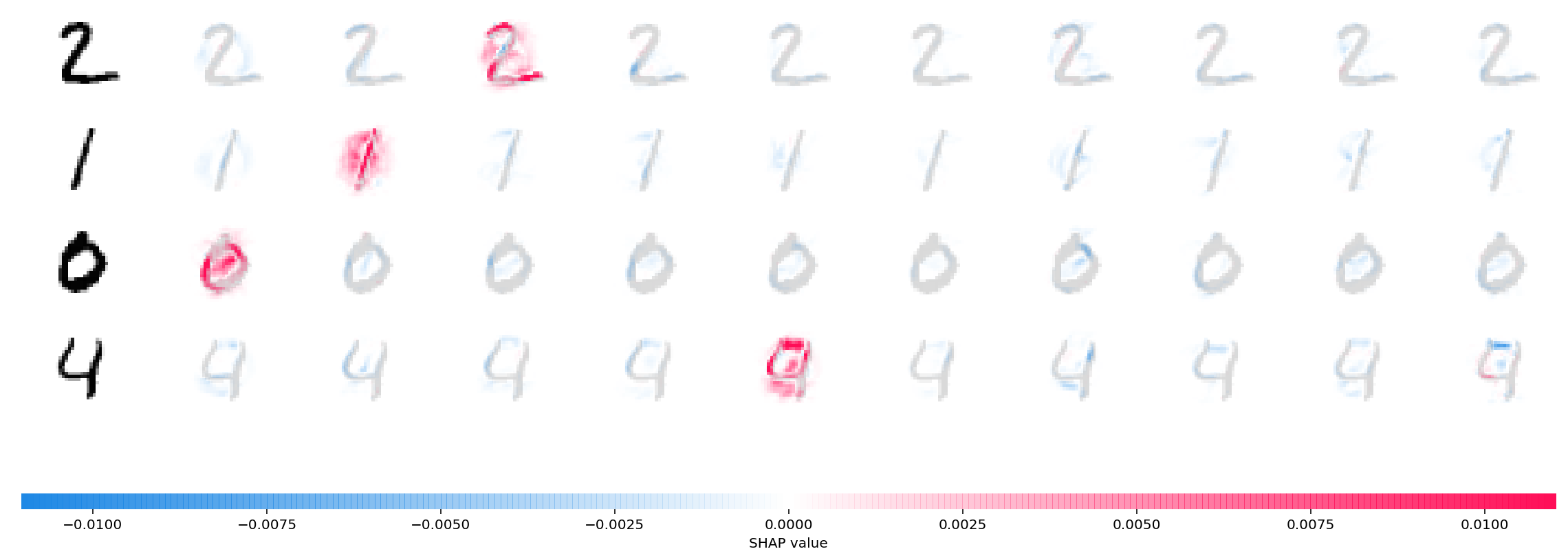
The plot above explains ten outputs (digits 0-9) for four different images. Red pixels increase the model's output while blue pixels decrease the output. The input images are shown on the left, and as nearly transparent grayscale backings behind each of the explanations. The sum of the SHAP values equals the difference between the expected model output (averaged over the background dataset) and the current model output. Note that for the 'zero' image the blank middle is important, while for the 'four' image the lack of a connection on top makes it a four instead of a nine.

Deep learning example with GradientExplainer (TensorFlow/Keras/PyTorch models)

Expected gradients combines ideas from Integrated Gradients, SHAP, and SmoothGrad into a single expected value equation. This allows an entire dataset to be used as the background distribution (as opposed to a single reference value) and allows local smoothing. If we approximate the model with a linear function between each background data sample and the current input to be explained, and we assume the input features are independent then expected gradients will compute approximate SHAP values. In the example below we have explained how the 7th intermediate layer of the VGG16 ImageNet model impacts the output probabilities.

from keras.applications.vgg16 import VGG16
from keras.applications.vgg16 import preprocess_input
import keras.backend as K
import numpy as np
import json
import shap

# load pre-trained model and choose two images to explain
model = VGG16(weights='imagenet', include_top=True)
X,y = shap.datasets.imagenet50()
to_explain = X[[39,41]]

# load the ImageNet class names
url = "https://s3.amazonaws.com/deep-learning-models/image-models/imagenet_class_index.json"
fname = shap.datasets.cache(url)
with open(fname) as f:
    class_names = json.load(f)

# explain how the input to the 7th layer of the model explains the top two classes
def map2layer(x, layer):
    feed_dict = dict(zip([model.layers[0].input], [preprocess_input(x.copy())]))
    return K.get_session().run(model.layers[layer].input, feed_dict)
e = shap.GradientExplainer(
    (model.layers[7].input, model.layers[-1].output),
    map2layer(X, 7),
    local_smoothing=0 # std dev of smoothing noise
)
shap_values,indexes = e.shap_values(map2layer(to_explain, 7), ranked_outputs=2)

# get the names for the classes
index_names = np.vectorize(lambda x: class_names[str(x)][1])(indexes)

# plot the explanations
shap.image_plot(shap_values, to_explain, index_names)

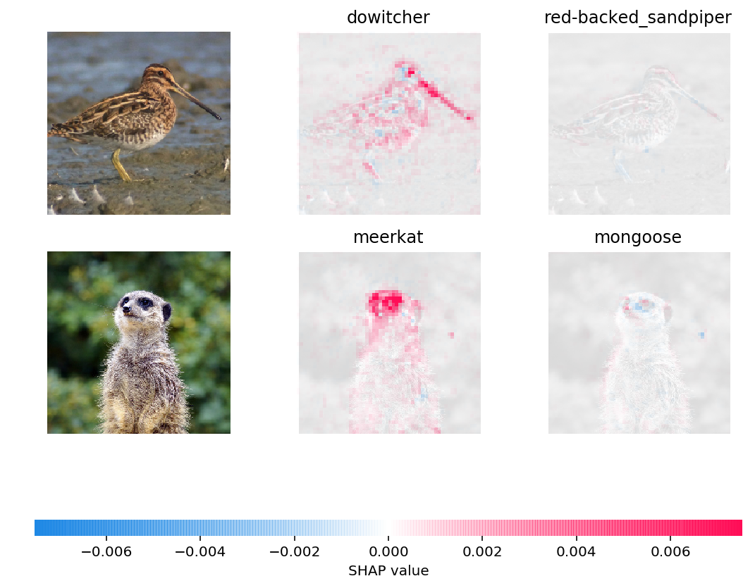
Predictions for two input images are explained in the plot above. Red pixels represent positive SHAP values that increase the probability of the class, while blue pixels represent negative SHAP values the reduce the probability of the class. By using ranked_outputs=2 we explain only the two most likely classes for each input (this spares us from explaining all 1,000 classes).

Model agnostic example with KernelExplainer (explains any function)

Kernel SHAP uses a specially-weighted local linear regression to estimate SHAP values for any model. Below is a simple example for explaining a multi-class SVM on the classic iris dataset.

import sklearn
import shap
from sklearn.model_selection import train_test_split

# print the JS visualization code to the notebook
shap.initjs()

# train a SVM classifier
X_train,X_test,Y_train,Y_test = train_test_split(*shap.datasets.iris(), test_size=0.2, random_state=0)
svm = sklearn.svm.SVC(kernel='rbf', probability=True)
svm.fit(X_train, Y_train)

# use Kernel SHAP to explain test set predictions
explainer = shap.KernelExplainer(svm.predict_proba, X_train, link="logit")
shap_values = explainer.shap_values(X_test, nsamples=100)

# plot the SHAP values for the Setosa output of the first instance
shap.force_plot(explainer.expected_value[0], shap_values[0][0,:], X_test.iloc[0,:], link="logit")

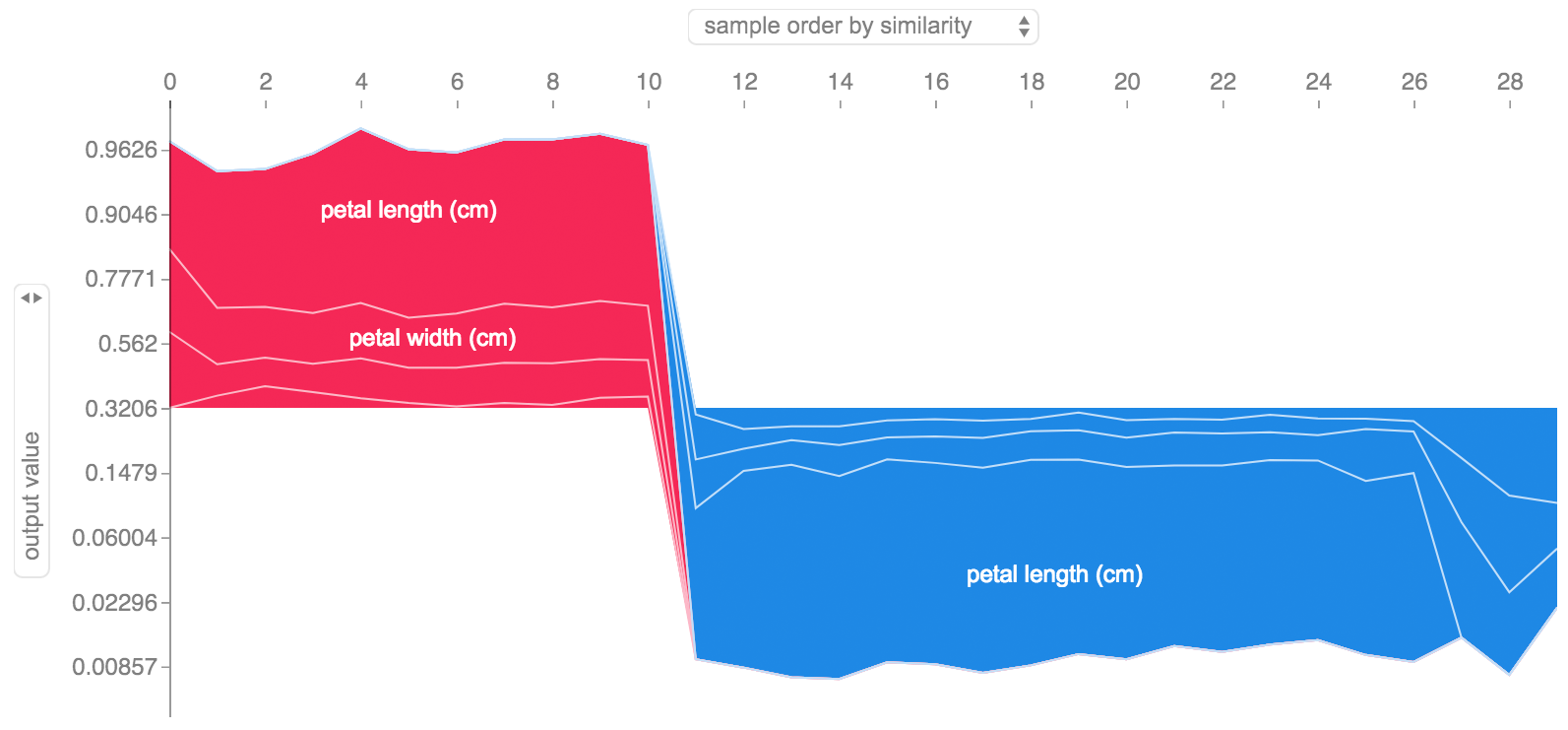
The above explanation shows four features each contributing to push the model output from the base value (the average model output over the training dataset we passed) towards zero. If there were any features pushing the class label higher they would be shown in red.

If we take many explanations such as the one shown above, rotate them 90 degrees, and then stack them horizontally, we can see explanations for an entire dataset. This is exactly what we do below for all the examples in the iris test set:

# plot the SHAP values for the Setosa output of all instances
shap.force_plot(explainer.expected_value[0], shap_values[0], X_test, link="logit")

SHAP Interaction Values

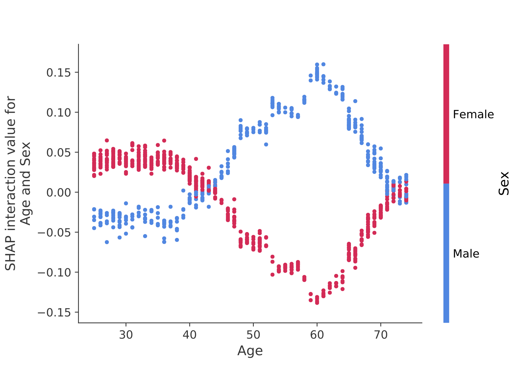
SHAP interaction values are a generalization of SHAP values to higher order interactions. Fast exact computation of pairwise interactions are implemented for tree models with shap.TreeExplainer(model).shap_interaction_values(X). This returns a matrix for every prediction, where the main effects are on the diagonal and the interaction effects are off-diagonal. These values often reveal interesting hidden relationships, such as how the increased risk of death peaks for men at age 60 (see the NHANES notebook for details):

Sample notebooks

The notebooks below demonstrate different use cases for SHAP. Look inside the notebooks directory of the repository if you want to try playing with the original notebooks yourself.

TreeExplainer

An implementation of Tree SHAP, a fast and exact algorithm to compute SHAP values for trees and ensembles of trees.

NHANES survival model with XGBoost and SHAP interaction values - Using mortality data from 20 years of followup this notebook demonstrates how to use XGBoost and shap to uncover complex risk factor relationships.
Census income classification with LightGBM - Using the standard adult census income dataset, this notebook trains a gradient boosting tree model with LightGBM and then explains predictions using shap.
League of Legends Win Prediction with XGBoost - Using a Kaggle dataset of 180,000 ranked matches from League of Legends we train and explain a gradient boosting tree model with XGBoost to predict if a player will win their match.

DeepExplainer

An implementation of Deep SHAP, a faster (but only approximate) algorithm to compute SHAP values for deep learning models that is based on connections between SHAP and the DeepLIFT algorithm.

MNIST Digit classification with Keras - Using the MNIST handwriting recognition dataset, this notebook trains a neural network with Keras and then explains predictions using shap.
Keras LSTM for IMDB Sentiment Classification - This notebook trains an LSTM with Keras on the IMDB text sentiment analysis dataset and then explains predictions using shap.

GradientExplainer

An implementation of expected gradients to approximate SHAP values for deep learning models. It is based on connections between SHAP and the Integrated Gradients algorithm. GradientExplainer is slower than DeepExplainer and makes different approximation assumptions.

Explain an Intermediate Layer of VGG16 on ImageNet - This notebook demonstrates how to explain the output of a pre-trained VGG16 ImageNet model using an internal convolutional layer.

LinearExplainer

For a linear model with independent features we can analytically compute the exact SHAP values. We can also account for feature correlation if we are willing to estimate the feature covariance matrix. LinearExplainer supports both of these options.

Sentiment Analysis with Logistic Regression - This notebook demonstrates how to explain a linear logistic regression sentiment analysis model.

KernelExplainer

An implementation of Kernel SHAP, a model agnostic method to estimate SHAP values for any model. Because it makes no assumptions about the model type, KernelExplainer is slower than the other model type specific algorithms.

Census income classification with scikit-learn - Using the standard adult census income dataset, this notebook trains a k-nearest neighbors classifier using scikit-learn and then explains predictions using shap.
ImageNet VGG16 Model with Keras - Explain the classic VGG16 convolutional neural network's predictions for an image. This works by applying the model agnostic Kernel SHAP method to a super-pixel segmented image.
Iris classification - A basic demonstration using the popular iris species dataset. It explains predictions from six different models in scikit-learn using shap.

Documentation notebooks

These notebooks comprehensively demonstrate how to use specific functions and objects.

Methods Unified by SHAP

LIME: Ribeiro, Marco Tulio, Sameer Singh, and Carlos Guestrin. "Why should i trust you?: Explaining the predictions of any classifier." Proceedings of the 22nd ACM SIGKDD International Conference on Knowledge Discovery and Data Mining. ACM, 2016.
Shapley sampling values: Strumbelj, Erik, and Igor Kononenko. "Explaining prediction models and individual predictions with feature contributions." Knowledge and information systems 41.3 (2014): 647-665.
DeepLIFT: Shrikumar, Avanti, Peyton Greenside, and Anshul Kundaje. "Learning important features through propagating activation differences." arXiv preprint arXiv:1704.02685 (2017).
QII: Datta, Anupam, Shayak Sen, and Yair Zick. "Algorithmic transparency via quantitative input influence: Theory and experiments with learning systems." Security and Privacy (SP), 2016 IEEE Symposium on. IEEE, 2016.
Layer-wise relevance propagation: Bach, Sebastian, et al. "On pixel-wise explanations for non-linear classifier decisions by layer-wise relevance propagation." PloS one 10.7 (2015): e0130140.
Shapley regression values: Lipovetsky, Stan, and Michael Conklin. "Analysis of regression in game theory approach." Applied Stochastic Models in Business and Industry 17.4 (2001): 319-330.
Tree interpreter: Saabas, Ando. Interpreting random forests. http://blog.datadive.net/interpreting-random-forests/

Citations

The algorithms and visualizations used in this package came primarily out of research in Su-In Lee's lab at the University of Washington, and Microsoft Research. If you use SHAP in your research we would appreciate a citation to the appropriate paper(s):

For general use of SHAP you can read/cite our NeurIPS paper (bibtex).
For TreeExplainer you can read/cite our Nature Machine Intelligence paper (bibtex; free access).
For GPUTreeExplainer you can read/cite this article.
For force_plot visualizations and medical applications you can read/cite our Nature Biomedical Engineering paper (bibtex; free access).

Project details

These details have not been verified by PyPI

Project links

Release history Release notifications | RSS feed

This version

0.51.0

Mar 4, 2026

0.50.0

Nov 11, 2025

0.49.1

Oct 14, 2025

0.48.0

Jun 12, 2025

0.47.2

Apr 17, 2025

0.47.1

Mar 22, 2025

0.47.0

Mar 5, 2025

0.46.0

Jun 27, 2024

0.45.1

May 7, 2024

0.45.0

Mar 8, 2024

0.44.1

Jan 25, 2024

0.44.0

Dec 7, 2023

0.43.0

Oct 9, 2023

0.42.1

Jul 15, 2023

0.42.0

Jul 6, 2023

0.41.0

Jun 16, 2022

0.40.0

Oct 20, 2021

0.39.0

Mar 3, 2021

0.38.1

Jan 15, 2021

0.37.0

Nov 4, 2020

0.36.0

Aug 27, 2020

0.35.0

Feb 27, 2020

0.34.0

Dec 27, 2019

0.33.0

Dec 11, 2019

0.32.1

Nov 6, 2019

0.32.0

Nov 6, 2019

0.31.0

Oct 21, 2019

0.30.2

Sep 30, 2019

0.30.1

Sep 9, 2019

0.30.0

Aug 31, 2019

0.29.3

Jun 19, 2019

0.29.2

Jun 19, 2019

0.29.1

May 15, 2019

0.28.6

May 14, 2019

0.28.5

Feb 16, 2019

0.28.4

Feb 16, 2019

0.28.3

Jan 24, 2019

0.28.2

Jan 23, 2019

0.28.1

Jan 23, 2019

0.28.0

Jan 21, 2019

0.27.0

Jan 1, 2019

0.26.0

Dec 12, 2018

0.25.2

Nov 9, 2018

0.25.1

Nov 8, 2018

0.25.0

Nov 7, 2018

0.24.0

Aug 24, 2018

0.23.2

Aug 24, 2018

0.23.1

Aug 16, 2018

0.23.0

Aug 16, 2018

0.22.3

Aug 9, 2018

0.22.2

Aug 8, 2018

0.22.1

Aug 8, 2018

0.22.0

Aug 8, 2018

0.21.0

Jul 24, 2018

0.20.2

Jul 23, 2018

0.20.1

Jul 17, 2018

0.19.5

Jul 13, 2018

0.19.4

Jul 12, 2018

0.19.3

Jul 7, 2018

0.19.2

Jun 29, 2018

0.19.1

Jun 28, 2018

0.18.1

Jun 7, 2018

0.18.0

Jun 7, 2018

0.17.1

May 30, 2018

0.17.0

May 29, 2018

0.16.1

May 21, 2018

0.15.0

May 3, 2018

0.14.1

Apr 19, 2018

0.14.0

Apr 14, 2018

0.13.7

Apr 12, 2018

0.13.6

Apr 11, 2018

0.13.5

Apr 11, 2018

0.13.3

Apr 10, 2018

0.13.2

Apr 10, 2018

0.13.1

Apr 10, 2018

0.13

Apr 9, 2018

0.12.1

Apr 5, 2018

0.12.0

Mar 22, 2018

0.11.1

Mar 7, 2018

0.11.0

Mar 3, 2018

0.10.3

Feb 20, 2018

0.10.2

Feb 19, 2018

0.10.1

Feb 15, 2018

0.10.0

Feb 13, 2018

0.9.1

Feb 12, 2018

0.8.9

Feb 7, 2018

0.8.8

Feb 5, 2018

0.8.7

Feb 2, 2018

0.8.6

Feb 1, 2018

0.8.5

Jan 31, 2018

0.8.4

Jan 31, 2018

0.8.3

Jan 29, 2018

0.8.2

Jan 29, 2018

0.8.1

Jan 29, 2018

0.8.0

Jan 23, 2018

0.7.0

Dec 7, 2017

0.6.1

Dec 1, 2017

0.6

Nov 23, 2017

0.5

Oct 25, 2017

0.3.3

Oct 4, 2017

0.3.2

Oct 3, 2017

0.3.1

Sep 26, 2017

0.3

Sep 21, 2017

0.2.4

May 18, 2017

0.2.3

Apr 18, 2017

0.2.2

Apr 14, 2017

0.2.1

Dec 9, 2016

0.2

Dec 1, 2016

0.1.2

Dec 1, 2016

0.1

Dec 1, 2016

Download files

Download the file for your platform. If you're not sure which to choose, learn more about installing packages.

Source Distribution

shap-0.51.0.tar.gz (4.1 MB view details)

Uploaded Mar 4, 2026 Source

Built Distributions

If you're not sure about the file name format, learn more about wheel file names.

The dropdown lists show the available interpreters, ABIs, and platforms. Enable javascript to be able to filter the list of wheel files.

shap-0.51.0-cp314-cp314t-musllinux_1_2_x86_64.whl (2.1 MB view details)

Uploaded Mar 4, 2026 CPython 3.14tmusllinux: musl 1.2+ x86-64

shap-0.51.0-cp314-cp314t-musllinux_1_2_aarch64.whl (2.0 MB view details)

Uploaded Mar 4, 2026 CPython 3.14tmusllinux: musl 1.2+ ARM64

shap-0.51.0-cp314-cp314t-manylinux2014_aarch64.manylinux_2_17_aarch64.manylinux_2_28_aarch64.whl (1.1 MB view details)

Uploaded Mar 4, 2026 CPython 3.14tmanylinux: glibc 2.17+ ARM64manylinux: glibc 2.28+ ARM64

shap-0.51.0-cp314-cp314t-macosx_11_0_arm64.whl (568.9 kB view details)

Uploaded Mar 4, 2026 CPython 3.14tmacOS 11.0+ ARM64

shap-0.51.0-cp314-cp314-win_amd64.whl (559.2 kB view details)

Uploaded Mar 4, 2026 CPython 3.14Windows x86-64

shap-0.51.0-cp314-cp314-musllinux_1_2_x86_64.whl (2.1 MB view details)

Uploaded Mar 4, 2026 CPython 3.14musllinux: musl 1.2+ x86-64

shap-0.51.0-cp314-cp314-musllinux_1_2_aarch64.whl (2.0 MB view details)

Uploaded Mar 4, 2026 CPython 3.14musllinux: musl 1.2+ ARM64

shap-0.51.0-cp314-cp314-manylinux2014_x86_64.manylinux_2_17_x86_64.manylinux_2_28_x86_64.whl (1.1 MB view details)

Uploaded Mar 4, 2026 CPython 3.14manylinux: glibc 2.17+ x86-64manylinux: glibc 2.28+ x86-64

shap-0.51.0-cp314-cp314-manylinux2014_aarch64.manylinux_2_17_aarch64.manylinux_2_28_aarch64.whl (1.1 MB view details)

Uploaded Mar 4, 2026 CPython 3.14manylinux: glibc 2.17+ ARM64manylinux: glibc 2.28+ ARM64

shap-0.51.0-cp314-cp314-macosx_11_0_arm64.whl (562.4 kB view details)

Uploaded Mar 4, 2026 CPython 3.14macOS 11.0+ ARM64

shap-0.51.0-cp313-cp313-win_amd64.whl (555.9 kB view details)

Uploaded Mar 4, 2026 CPython 3.13Windows x86-64

shap-0.51.0-cp313-cp313-musllinux_1_2_x86_64.whl (2.1 MB view details)

Uploaded Mar 4, 2026 CPython 3.13musllinux: musl 1.2+ x86-64

shap-0.51.0-cp313-cp313-musllinux_1_2_aarch64.whl (2.0 MB view details)

Uploaded Mar 4, 2026 CPython 3.13musllinux: musl 1.2+ ARM64

shap-0.51.0-cp313-cp313-manylinux2014_x86_64.manylinux_2_17_x86_64.manylinux_2_28_x86_64.whl (1.1 MB view details)

Uploaded Mar 4, 2026 CPython 3.13manylinux: glibc 2.17+ x86-64manylinux: glibc 2.28+ x86-64

shap-0.51.0-cp313-cp313-manylinux2014_aarch64.manylinux_2_17_aarch64.manylinux_2_28_aarch64.whl (1.1 MB view details)

Uploaded Mar 4, 2026 CPython 3.13manylinux: glibc 2.17+ ARM64manylinux: glibc 2.28+ ARM64

shap-0.51.0-cp313-cp313-macosx_11_0_arm64.whl (561.7 kB view details)

Uploaded Mar 4, 2026 CPython 3.13macOS 11.0+ ARM64

shap-0.51.0-cp313-cp313-macosx_10_13_x86_64.whl (564.9 kB view details)

Uploaded Mar 4, 2026 CPython 3.13macOS 10.13+ x86-64

shap-0.51.0-cp312-cp312-win_amd64.whl (556.1 kB view details)

Uploaded Mar 4, 2026 CPython 3.12Windows x86-64

shap-0.51.0-cp312-cp312-musllinux_1_2_x86_64.whl (2.1 MB view details)

Uploaded Mar 4, 2026 CPython 3.12musllinux: musl 1.2+ x86-64

shap-0.51.0-cp312-cp312-musllinux_1_2_aarch64.whl (2.0 MB view details)

Uploaded Mar 4, 2026 CPython 3.12musllinux: musl 1.2+ ARM64

shap-0.51.0-cp312-cp312-manylinux2014_x86_64.manylinux_2_17_x86_64.manylinux_2_28_x86_64.whl (1.1 MB view details)

Uploaded Mar 4, 2026 CPython 3.12manylinux: glibc 2.17+ x86-64manylinux: glibc 2.28+ x86-64

shap-0.51.0-cp312-cp312-manylinux2014_aarch64.manylinux_2_17_aarch64.manylinux_2_28_aarch64.whl (1.1 MB view details)

Uploaded Mar 4, 2026 CPython 3.12manylinux: glibc 2.17+ ARM64manylinux: glibc 2.28+ ARM64

shap-0.51.0-cp312-cp312-macosx_11_0_arm64.whl (562.3 kB view details)

Uploaded Mar 4, 2026 CPython 3.12macOS 11.0+ ARM64

shap-0.51.0-cp312-cp312-macosx_10_13_x86_64.whl (565.7 kB view details)

Uploaded Mar 4, 2026 CPython 3.12macOS 10.13+ x86-64

shap-0.51.0-cp311-cp311-win_amd64.whl (554.9 kB view details)

Uploaded Mar 4, 2026 CPython 3.11Windows x86-64

shap-0.51.0-cp311-cp311-musllinux_1_2_x86_64.whl (2.1 MB view details)

Uploaded Mar 4, 2026 CPython 3.11musllinux: musl 1.2+ x86-64

shap-0.51.0-cp311-cp311-musllinux_1_2_aarch64.whl (2.0 MB view details)

Uploaded Mar 4, 2026 CPython 3.11musllinux: musl 1.2+ ARM64

shap-0.51.0-cp311-cp311-manylinux2014_x86_64.manylinux_2_17_x86_64.manylinux_2_28_x86_64.whl (1.1 MB view details)

Uploaded Mar 4, 2026 CPython 3.11manylinux: glibc 2.17+ x86-64manylinux: glibc 2.28+ x86-64

shap-0.51.0-cp311-cp311-manylinux2014_aarch64.manylinux_2_17_aarch64.manylinux_2_28_aarch64.whl (1.1 MB view details)

Uploaded Mar 4, 2026 CPython 3.11manylinux: glibc 2.17+ ARM64manylinux: glibc 2.28+ ARM64

shap-0.51.0-cp311-cp311-macosx_11_0_arm64.whl (562.8 kB view details)

Uploaded Mar 4, 2026 CPython 3.11macOS 11.0+ ARM64

shap-0.51.0-cp311-cp311-macosx_10_9_x86_64.whl (565.1 kB view details)

Uploaded Mar 4, 2026 CPython 3.11macOS 10.9+ x86-64

File details

Details for the file shap-0.51.0.tar.gz.

File metadata

Download URL: shap-0.51.0.tar.gz
Upload date: Mar 4, 2026
Size: 4.1 MB
Tags: Source
Uploaded using Trusted Publishing? Yes
Uploaded via: twine/6.1.0 CPython/3.13.7

File hashes

Hashes for shap-0.51.0.tar.gz
Algorithm	Hash digest
SHA256	`cfa17ff213657c9d50285aa923d79b0037a62e2ee1a31bc3eec7e196b00bdb59`
MD5	`9fa2da92bf7711ce2d775b46b3fd637d`
BLAKE2b-256	`a40a4a3ee4b1a3654f2a9ae038a64bb3e91a42af3da07577d69b65241f010970`

Algorithm	Hash digest
SHA256	`23c33eae29f887153ef952846ec3bff6abc0aed3aa01594e4ae66cd94a227a49`
MD5	`91d3f0d052479f5bed060a8323a49b14`
BLAKE2b-256	`d6423668db63cb38e9648e97087d60a0d4ce569c2e8c2b8828124e6da433026f`

Algorithm	Hash digest
SHA256	`71e18a6850af4cdeece1a3f9d4b633a421885fcfda079125e3d35ea08433d3eb`
MD5	`44645bcc8447c127899e10eec7c24bd9`
BLAKE2b-256	`12d13f7b841dd943a1cbb9c693ed65366c6afc1ac54c70065e0281fa82b57075`

Algorithm	Hash digest
SHA256	`18828bc4f78adb644ae35c50e79a246d262fa6cf17143c78cca091796b21c27b`
MD5	`1f18c3687f7f9fe2970baa6b9289247d`
BLAKE2b-256	`a61604467bf7b8430c3a5c709401ab065022a72340bc50dfaf67a1cc117ce15e`

Algorithm	Hash digest
SHA256	`80132eca5679e7e8da7a0d9bfee58d0a3979be25630fd6598ef608bbcefce784`
MD5	`70f2d68cf8fb460d102ef0744b4bac0c`
BLAKE2b-256	`d2568c5f94ae86590e612487c77b9b9bef3fd2f3c91969b3c6e8743ce06440f3`

Algorithm	Hash digest
SHA256	`86f24dab2c64d78f38170d490a03ff6fb1b48cf3bd0a1527e9bed23e74ad5d2c`
MD5	`d7c91caded7528eb8715c14c8086668e`
BLAKE2b-256	`6a5e60fbf1ffe0c150c4db0e80e31b3f9428e633d33ccf072e1e75227679cbfc`

Algorithm	Hash digest
SHA256	`c52aa8fb311502d5d25e8d631806326656318ab4094459ddbf1410837aaeb139`
MD5	`fe0096537fc72333b3eac84aabfb1e2a`
BLAKE2b-256	`aa38a25863c3c8d344e3e322b8dcbac41929b9d00cfb9df3166ac9c350d89c53`

Algorithm	Hash digest
SHA256	`331d80a993e32404dd76254f5a82cb481453b4d9e58c0e7da13a3b700a381b03`
MD5	`ca9e2406b4bebf8a94737490fdd332e0`
BLAKE2b-256	`e8c345ab3242f055980938671d568540ff1dbd84eb9bf4fe0d3235432f7bad35`

Algorithm	Hash digest
SHA256	`da930d73fa23d7a296660431f01726ae47ef2e7d9fee7e1632fb674be7b150b9`
MD5	`ae1d96b729e108d40e80574d4fb77d66`
BLAKE2b-256	`3181cf180b20ac0c1323b78386667a24dfc2f6d827baa0b223d84bfd5818aa03`

Algorithm	Hash digest
SHA256	`6afaeac1fdd7883a058fb071c7044aff6c44699377a35a5d73e75b68564d0d47`
MD5	`aa8942fd956aa63673bafb2b72336856`
BLAKE2b-256	`8cc8c3b067d10c7a792fd1a32ea93f218b2c217fa99d125f79f26d31376ae246`

Algorithm	Hash digest
SHA256	`d0c33498ed7042f7259ff207bd3aa1cc814fb759240e5f1500e018660b597c17`
MD5	`82f7a41207c7de97d6049c218bc7546c`
BLAKE2b-256	`1f57f48dd00ac0d9f75a1f34f5ae47ed3269e8acd541189555f39e49e6f126f4`

Algorithm	Hash digest
SHA256	`5f51ca55bda10b3fa2125f2b8e08e9d6a6edcbb0e752c67050e87a6d3ca7d53b`
MD5	`536669a2e4b841c8791d5c977a01dd4d`
BLAKE2b-256	`79d51ec3120f461f31a03d1d2f1d339f5058f12c7a542d22bfcc350511eccc8a`

Algorithm	Hash digest
SHA256	`f461e5a1d6b0cae3fd9c6bd00c95111ed95b9e0020ec71f14291429ed17d49f4`
MD5	`950d26d5dd1b9b0ede7a054ace7fc36c`
BLAKE2b-256	`f365b95588a1f48eb9e98aa61e6db31cf63a388970e4c11341d40ddece3b54f8`

Algorithm	Hash digest
SHA256	`33540a7e3c70bd1a742a4d0576c19b5e000165038de953d3ebf31a7bb53d01f4`
MD5	`a1985956b06df7b7379133dc734cf507`
BLAKE2b-256	`c68e9072acfcbe6abc79fbfe87360c7dcfe16d7498cdb13dc560820912eb5dd5`

Algorithm	Hash digest
SHA256	`f32d006680708513efff07f67dcbe44a531b242ae042dee99b7024e210391ac2`
MD5	`5a375edd6d55d970c644cd28d1f4a072`
BLAKE2b-256	`64b1472ca0adf25215dfdbca9f398d853536413091fe47dd69bb3f67dbd445f4`

Algorithm	Hash digest
SHA256	`13eb21626ea671604769c847ac0604871a03df0842522087ffc00181683780a4`
MD5	`6e54cf791ead62899ce60392642f5210`
BLAKE2b-256	`ecb776dbca9c4b83602841c016fec7201e4146c5e6347a8b0428e7c0617ba424`

Algorithm	Hash digest
SHA256	`724cdd8298450ae22b08ca40e07136c73e4e75dbdf8e3f07d741a291bf636dad`
MD5	`0c6cd15e66ffb03e86b12ad283499f5d`
BLAKE2b-256	`e65e5c6d37992e93b3fa44509d8544281cd5ae357c8946bc0e756e78139b4baf`

Algorithm	Hash digest
SHA256	`f3efeef8a76e2ee735fad50f82e5a8e56ba8639f42e2fa50dc1997caed77c488`
MD5	`882b46b4dfafe4698d89b0354117a9c0`
BLAKE2b-256	`364a77f8dc2c6874d8a27123afffcb79f540a80ed3ccfd640604e4d8beb9cc5e`

Algorithm	Hash digest
SHA256	`ee76aa705927ac64acd4f506722f52596e77d3ced87078bc86bfcb4571c7b976`
MD5	`73ca7193a7296315feaf2e5e5ff4ca40`
BLAKE2b-256	`200e6f581645b66efff6bf091953f474eb16e64da499cfac0c552dd77559f205`

Algorithm	Hash digest
SHA256	`c3b878f6414213a12247faa00d609957fdfbcc33cfd48a6751500c4708b5666d`
MD5	`5f40967bf0b98e4c353601b2496f7ba8`
BLAKE2b-256	`c9fd9b295ad15420566dca713b792d9beb65692804b96c69cc99ffec5e31db58`

Algorithm	Hash digest
SHA256	`dee16e81082dec5ce2a37c41c2b9cbebcb4bf7de79133a72d84a4093b7d4158c`
MD5	`37c2dac3687929718cb12c8596d717d7`
BLAKE2b-256	`808938c903c438b33063b006f41d00684af8b424bb95f0fcfd8963d1501bf427`

shap 0.51.0

Navigation

Verified details

Maintainers

Unverified details

Project links

Meta

Classifiers

Project description

Install

Contributing

Tree ensemble example (XGBoost/LightGBM/CatBoost/scikit-learn/pyspark models)

Natural language example (transformers)

Deep learning example with DeepExplainer (TensorFlow/Keras models)

Deep learning example with GradientExplainer (TensorFlow/Keras/PyTorch models)

Model agnostic example with KernelExplainer (explains any function)

SHAP Interaction Values

Sample notebooks

TreeExplainer

DeepExplainer

GradientExplainer

LinearExplainer

KernelExplainer

Documentation notebooks

Methods Unified by SHAP

Citations

Project details

Verified details

Maintainers

Unverified details

Project links

Meta

Classifiers

Release history Release notifications | RSS feed

Download files

Source Distribution

Built Distributions

File details

File metadata

File hashes

Provenance

File details

File metadata

File hashes

Provenance

File details

File metadata

File hashes

Provenance

File details

File metadata

File hashes

Provenance

File details

File metadata

File hashes

Provenance

File details

File metadata

File hashes

Provenance

File details

File metadata

File hashes

Provenance

File details

File metadata

File hashes

Provenance

File details

File metadata

File hashes

Provenance

File details

File metadata

File hashes

Provenance

File details

File metadata

File hashes

Algorithm	Hash digest
SHA256	`0b1f9e62d6a3fa28765d7b61abda7caf76aba21e769423fbf3ce8a7a5e498243`
MD5	`944a05877149c3b5e27149e9fd87c67b`
BLAKE2b-256	`afc1a9152876b04f9a05ca18bd3e8bc4bc72468ae32429bfbb30a9cbd4ad35b9`

Algorithm	Hash digest
SHA256	`1aa9f659d2028e26ac7ec34cafbc14585fdc14d0c8973e9442c65af1af1ff781`
MD5	`f3f855f9c613edd2050bb4ac9d6a9223`
BLAKE2b-256	`93a137e7229be000cf608ece024dcd76edae4cc618b22b402ea78270849cac3f`

Algorithm	Hash digest
SHA256	`e412bb475c9074ffd6684abb88d86d93275729b344cbfb37b4e4db37db759fbf`
MD5	`4072c315bb76e6188f38145bcdeee6b6`
BLAKE2b-256	`49fd07f7c454ff5dff455576e5bb08cdb2cab05a4c1eb5e1b9959ef2ac28366d`

Algorithm	Hash digest
SHA256	`07b0367408b1b9fc51556f2ddac5ee4209cc51be592099e6d51d0834c9b037d8`
MD5	`2c94a20e3a9f9b26225c30fcda39790d`
BLAKE2b-256	`5aba8c8fac8506327febada7dc58f90dc459287995bb7b8aadbc44506e61be55`

Algorithm	Hash digest
SHA256	`ca2a9171e6c5b9a700d585982d7fd8336856ad818e24264420c56f9d8f02a961`
MD5	`bfd094581dd5d61c821e51956f34406b`
BLAKE2b-256	`a58ecee1ee136a4e54fe2fbb63a60d72d7c25e21a4ffe6aa05779cab7669cb31`

Algorithm	Hash digest
SHA256	`6f3a83f28d2304f81645392a1d346154d9d992705e762fb949fa5371925399b2`
MD5	`47940846a36d0b1f150c5ed6f302b228`
BLAKE2b-256	`72ac751f3070be48c4b365f565ca5b4ba4c93b0a371d8ee595859c62eab9885b`

Algorithm	Hash digest
SHA256	`ff5534e92f5876c74975b53cc6b251126bbe092e5032f81e1fe8583c4a74d58c`
MD5	`e309bce35d682903599a3ae412b68845`
BLAKE2b-256	`5ff902269c83b3056c5fbaa13911e59b844146ed80c97a6f78aa0d374a9e8368`

Algorithm	Hash digest
SHA256	`5a909d6e306d4083e4862b6d097d53f3b4aa4d5cdf2ef4dbac5e8245160d9abd`
MD5	`91f5c774b261359c1aa111e887f4fcc7`
BLAKE2b-256	`4248541bd5b7f068804f33fac459274c06a46deb8f0e1edf3a9b176c00137629`

Algorithm	Hash digest
SHA256	`3ddd314c9dc766f72027b3b6d9a8b975c7df67f1a27af7f857267c716b7d3dd8`
MD5	`bf0333dbce7d2064660a3110c02c1520`
BLAKE2b-256	`fc09a952ef8a1fe64b8a7bb909b2d3ab614d33cff7fdf646d62c3bd35d84de02`

Algorithm	Hash digest
SHA256	`9b92f7371644c4a19660f734e0b0fe299d0eff273102230c9cf191e310576619`
MD5	`36c658b1b96d0891409fa6d349fc10f2`
BLAKE2b-256	`14bfbafa92ae6606f1ee38f14e866045fbcae21412a3a5766fb493b951a6e6e1`