The Clusters-Features package allows data science users to compute high-level linear algebra operations on any type of data set.

Project description
Clusters-Features : a Python module to evaluate the quality of clustering

This package is made for unsupervised learning. All criterias are used with internal validation and make no use of ground-truth labels.
Official documentation : simonbertrand.pages.unistra.fr/Clusters-Features
Table of contents
Introduction
Clusters-Features is a package that computes many operations using only the dataset and the target vector.
Data
The package provides all the usefull data such as pairwise distances or distances between every elements and the centroid of given cluster. You can also check for the maximum/minimum distances between two elements of different clusters or even each intercentroid distances. But you can also get different radius for each centroids and analyse them to firstly understand the shape of the clusters. The distribution of all radius for each cluster is also available. All informative data is contained inside the subclass Data.
Score
Approximatively 40 different internal indices have been implemented in Python : Ball-Hall Index, Dunn Index, Generalized Dunn Indexes (18 indexes), C Index, Banfeld-Raftery Index, Davies-Bouldin Index, Calinski-Harabasz Index, Ray-Turi Index, Xie-Beni Index, Ratkowsky Lance Index, SD Index, Mclain Rao Index, Scott-Symons Index, PBM Index, Point biserial Index, Det Ratio Index, Log SumSquare Ratio Index, Wemmert-Gançarski Index. We use two systems to generate these index, the first is caching each computed index and the other directly compute them.
All these score are defined in the main reference, check for the Score section to find the reference.
Confusion Hypersphere
Clusters-Features also provides a deep analysis of the multidimensionnal space. Confusion Hypersphere consists of counting the number of element contained in several hyperspheres centered on different positions and with different radius. This feature allows users to understand which clusters are confused (in the sense of the Euclidean norm) with other clusters. These indicators make it possible to determine which clusters are the most separated from the others and this is clearly adapted to convex clusters since the hypersphere is convex.
Info
Info gives two kind of boards such as clusters board which gives you information for each clusters. The general board gives informations at a general scale of the dataset .
Density
This section uses a meshgrid to estimate a density by summing n-dim (for n=2 or n=3) Gaussian distrubution centred on each dataset points. We put the minimum contour as a given percentile of the current density. If percentile is 99% then only 1% of the highest density values will be retained. We can make it for 2D grid or 3D grid but it is quickly limited due to the large number of combinations needed to generate an n-dim grid.
Utils
Implement external packages and utils to the current dataset.
Graph (Falcutative)
Graph allows users to plot few kind of data generated by Clusters-Features. As Plotly is used to plot, this section is facultative in the case where user only need to get the different data and matrix to plot with their own module. In order to disable this section, you will have to go to settings.py and put to False the variable "Activated_Graph" and then re-build the package using setuptools. All requirements.txt are going to be generated in consequences of these settings.
Dependencies
Native dependencies :
Falcultative dependencies (may cause errors if the user forces the use of the method of these falcultative dependencies without having installed the correct libraries) :
- Graph : Plotly
- Utils : umap-learn, Numba, statsmodels
Graph is dependent of Utils to correctly work but the reciprocal is not true.
Command Line Interface
This package provides a command line interface that is available by running this command
python3 ./clustersfeatures-cli.py -h
The documentation for the CLI is contained inside the script. Just use --help arguments to understand what it does.
Import the module
from ClustersFeatures import *
Load a random data set
We choose here the scikit-learn digits data set because it is in high dimension (64) and has a large number of observations.
from sklearn.datasets import load_digits
import pandas as pd
digits = load_digits()
pd_df=pd.DataFrame(digits.data)
pd_df['target'] = digits.target
pd_df
| 0 | 1 | 2 | 3 | 4 | 5 | 6 | 7 | 8 | 9 | ... | 55 | 56 | 57 | 58 | 59 | 60 | 61 | 62 | 63 | target | |
|---|---|---|---|---|---|---|---|---|---|---|---|---|---|---|---|---|---|---|---|---|---|
| 0 | 0.0 | 0.0 | 5.0 | 13.0 | 9.0 | 1.0 | 0.0 | 0.0 | 0.0 | 0.0 | ... | 0.0 | 0.0 | 0.0 | 6.0 | 13.0 | 10.0 | 0.0 | 0.0 | 0.0 | 0 |
| 1 | 0.0 | 0.0 | 0.0 | 12.0 | 13.0 | 5.0 | 0.0 | 0.0 | 0.0 | 0.0 | ... | 0.0 | 0.0 | 0.0 | 0.0 | 11.0 | 16.0 | 10.0 | 0.0 | 0.0 | 1 |
| 2 | 0.0 | 0.0 | 0.0 | 4.0 | 15.0 | 12.0 | 0.0 | 0.0 | 0.0 | 0.0 | ... | 0.0 | 0.0 | 0.0 | 0.0 | 3.0 | 11.0 | 16.0 | 9.0 | 0.0 | 2 |
| 3 | 0.0 | 0.0 | 7.0 | 15.0 | 13.0 | 1.0 | 0.0 | 0.0 | 0.0 | 8.0 | ... | 0.0 | 0.0 | 0.0 | 7.0 | 13.0 | 13.0 | 9.0 | 0.0 | 0.0 | 3 |
| 4 | 0.0 | 0.0 | 0.0 | 1.0 | 11.0 | 0.0 | 0.0 | 0.0 | 0.0 | 0.0 | ... | 0.0 | 0.0 | 0.0 | 0.0 | 2.0 | 16.0 | 4.0 | 0.0 | 0.0 | 4 |
| ... | ... | ... | ... | ... | ... | ... | ... | ... | ... | ... | ... | ... | ... | ... | ... | ... | ... | ... | ... | ... | ... |
| 1792 | 0.0 | 0.0 | 4.0 | 10.0 | 13.0 | 6.0 | 0.0 | 0.0 | 0.0 | 1.0 | ... | 0.0 | 0.0 | 0.0 | 2.0 | 14.0 | 15.0 | 9.0 | 0.0 | 0.0 | 9 |
| 1793 | 0.0 | 0.0 | 6.0 | 16.0 | 13.0 | 11.0 | 1.0 | 0.0 | 0.0 | 0.0 | ... | 0.0 | 0.0 | 0.0 | 6.0 | 16.0 | 14.0 | 6.0 | 0.0 | 0.0 | 0 |
| 1794 | 0.0 | 0.0 | 1.0 | 11.0 | 15.0 | 1.0 | 0.0 | 0.0 | 0.0 | 0.0 | ... | 0.0 | 0.0 | 0.0 | 2.0 | 9.0 | 13.0 | 6.0 | 0.0 | 0.0 | 8 |
| 1795 | 0.0 | 0.0 | 2.0 | 10.0 | 7.0 | 0.0 | 0.0 | 0.0 | 0.0 | 0.0 | ... | 0.0 | 0.0 | 0.0 | 5.0 | 12.0 | 16.0 | 12.0 | 0.0 | 0.0 | 9 |
| 1796 | 0.0 | 0.0 | 10.0 | 14.0 | 8.0 | 1.0 | 0.0 | 0.0 | 0.0 | 2.0 | ... | 0.0 | 0.0 | 1.0 | 8.0 | 12.0 | 14.0 | 12.0 | 1.0 | 0.0 | 8 |
1797 rows × 65 columns
The important thing is that the given "pd_df" dataframe in the following argument has to be concatenated with the target vector. Then, just specify as second argument which column name has the target. The program is making automatically the separation :
CC=ClustersCharacteristics(pd_df,label_target="target")
Data tools
The ClustersCharacteristics object creates attributes that define clusters. We can find for example the barycenter.
CC.data_barycenter
0      0.000000
1      0.303840
2      5.204786
3     11.835838
4     11.848080
          ...
59    12.089037
60    11.809126
61     6.764051
62     2.067891
63     0.364496
Length: 64, dtype: float64
But also centroids, where the column j of the following matrix correspond to the coordinates of centroid of cluster j.
CC.data_centroids
| target | 0 | 1 | 2 | 3 | 4 | 5 | 6 | 7 | 8 | 9 |
|---|---|---|---|---|---|---|---|---|---|---|
| 0 | 0.000000 | 0.000000 | 0.000000 | 0.000000 | 0.000000 | 0.000000 | 0.000000 | 0.000000 | 0.000000 | 0.000000 |
| 1 | 0.022472 | 0.010989 | 0.932203 | 0.644809 | 0.000000 | 0.967033 | 0.000000 | 0.167598 | 0.143678 | 0.144444 |
| 2 | 4.185393 | 2.456044 | 9.666667 | 8.387978 | 0.453039 | 9.983516 | 1.138122 | 5.100559 | 5.022989 | 5.683333 |
| 3 | 13.095506 | 9.208791 | 14.186441 | 14.169399 | 7.055249 | 13.038462 | 11.165746 | 13.061453 | 11.603448 | 11.833333 |
| 4 | 11.297753 | 10.406593 | 9.627119 | 14.224044 | 11.497238 | 13.895604 | 9.585635 | 14.245810 | 12.402299 | 11.255556 |
| ... | ... | ... | ... | ... | ... | ... | ... | ... | ... | ... |
| 59 | 13.561798 | 9.137363 | 13.966102 | 14.650273 | 7.812155 | 14.736264 | 10.685083 | 11.659218 | 12.695402 | 12.044444 |
| 60 | 13.325843 | 13.027473 | 13.118644 | 13.972678 | 11.812155 | 9.362637 | 15.093923 | 2.206704 | 13.011494 | 13.144444 |
| 61 | 5.438202 | 8.576923 | 11.796610 | 8.672131 | 1.955801 | 2.532967 | 13.044199 | 0.011173 | 6.735632 | 8.894444 |
| 62 | 0.275281 | 3.049451 | 8.022599 | 1.409836 | 0.000000 | 0.197802 | 4.480663 | 0.000000 | 1.206897 | 2.094444 |
| 63 | 0.000000 | 1.494505 | 1.932203 | 0.065574 | 0.000000 | 0.000000 | 0.093923 | 0.000000 | 0.011494 | 0.055556 |
64 rows × 10 columns
We can show the list of clusters labels :
CC.labels_clusters
array([0, 1, 2, 3, 4, 5, 6, 7, 8, 9])
And look for the data with the same label target. For example we take here the first cluster label of the above list.
Cluster=CC.labels_clusters[0]
CC.data_clusters[Cluster]
| 0 | 1 | 2 | 3 | 4 | 5 | 6 | 7 | 8 | 9 | ... | 54 | 55 | 56 | 57 | 58 | 59 | 60 | 61 | 62 | 63 | |
|---|---|---|---|---|---|---|---|---|---|---|---|---|---|---|---|---|---|---|---|---|---|
| 0 | 0.0 | 0.0 | 5.0 | 13.0 | 9.0 | 1.0 | 0.0 | 0.0 | 0.0 | 0.0 | ... | 0.0 | 0.0 | 0.0 | 0.0 | 6.0 | 13.0 | 10.0 | 0.0 | 0.0 | 0.0 |
| 10 | 0.0 | 0.0 | 1.0 | 9.0 | 15.0 | 11.0 | 0.0 | 0.0 | 0.0 | 0.0 | ... | 0.0 | 0.0 | 0.0 | 0.0 | 1.0 | 10.0 | 13.0 | 3.0 | 0.0 | 0.0 |
| 20 | 0.0 | 0.0 | 3.0 | 13.0 | 11.0 | 7.0 | 0.0 | 0.0 | 0.0 | 0.0 | ... | 1.0 | 0.0 | 0.0 | 0.0 | 2.0 | 12.0 | 13.0 | 4.0 | 0.0 | 0.0 |
| 30 | 0.0 | 0.0 | 10.0 | 14.0 | 11.0 | 3.0 | 0.0 | 0.0 | 0.0 | 4.0 | ... | 0.0 | 0.0 | 0.0 | 0.0 | 11.0 | 16.0 | 12.0 | 3.0 | 0.0 | 0.0 |
| 36 | 0.0 | 0.0 | 6.0 | 14.0 | 10.0 | 2.0 | 0.0 | 0.0 | 0.0 | 0.0 | ... | 0.0 | 0.0 | 0.0 | 0.0 | 7.0 | 16.0 | 11.0 | 1.0 | 0.0 | 0.0 |
| ... | ... | ... | ... | ... | ... | ... | ... | ... | ... | ... | ... | ... | ... | ... | ... | ... | ... | ... | ... | ... | ... |
| 1739 | 0.0 | 0.0 | 10.0 | 11.0 | 7.0 | 0.0 | 0.0 | 0.0 | 0.0 | 4.0 | ... | 1.0 | 0.0 | 0.0 | 0.0 | 7.0 | 12.0 | 8.0 | 0.0 | 0.0 | 0.0 |
| 1745 | 0.0 | 0.0 | 7.0 | 14.0 | 8.0 | 4.0 | 0.0 | 0.0 | 0.0 | 0.0 | ... | 0.0 | 0.0 | 0.0 | 0.0 | 6.0 | 13.0 | 7.0 | 0.0 | 0.0 | 0.0 |
| 1746 | 0.0 | 0.0 | 9.0 | 15.0 | 6.0 | 0.0 | 0.0 | 0.0 | 0.0 | 2.0 | ... | 1.0 | 0.0 | 0.0 | 0.0 | 8.0 | 15.0 | 11.0 | 4.0 | 0.0 | 0.0 |
| 1768 | 0.0 | 0.0 | 5.0 | 16.0 | 10.0 | 0.0 | 0.0 | 0.0 | 0.0 | 0.0 | ... | 5.0 | 0.0 | 0.0 | 0.0 | 4.0 | 15.0 | 16.0 | 8.0 | 1.0 | 0.0 |
| 1793 | 0.0 | 0.0 | 6.0 | 16.0 | 13.0 | 11.0 | 1.0 | 0.0 | 0.0 | 0.0 | ... | 1.0 | 0.0 | 0.0 | 0.0 | 6.0 | 16.0 | 14.0 | 6.0 | 0.0 | 0.0 |
178 rows × 64 columns
Users are able to get a pairwise distance matrix generated by the Scipy library (fast). If (xi,j)i,j is the returned matrix, then xi,j is the distance between element of index i and element of index j. The matrix is symetric as we use Euclidian norm to evaluate distances.
CC.data_every_element_distance_to_every_element
| 0 | 1 | 2 | 3 | 4 | 5 | 6 | 7 | 8 | 9 | ... | 1787 | 1788 | 1789 | 1790 | 1791 | 1792 | 1793 | 1794 | 1795 | 1796 | |
|---|---|---|---|---|---|---|---|---|---|---|---|---|---|---|---|---|---|---|---|---|---|
| 0 | 0.000000 | 59.556696 | 54.129474 | 47.571000 | 50.338852 | 43.908997 | 48.559242 | 56.000000 | 44.395946 | 40.804412 | ... | 39.874804 | 49.749372 | 52.640289 | 51.458721 | 49.989999 | 36.249138 | 26.627054 | 50.378567 | 37.067506 | 47.031904 |
| 1 | 59.556696 | 0.000000 | 41.629317 | 45.475268 | 47.906158 | 47.127487 | 40.286474 | 50.960769 | 48.620983 | 52.820451 | ... | 52.009614 | 48.969378 | 42.965102 | 32.572995 | 47.707442 | 51.390661 | 59.177699 | 38.587563 | 48.569538 | 50.328918 |
| 2 | 54.129474 | 41.629317 | 0.000000 | 53.953684 | 52.096065 | 55.443665 | 45.650849 | 49.335586 | 42.602817 | 54.836119 | ... | 59.076222 | 47.927028 | 46.335731 | 39.191836 | 46.936127 | 51.826634 | 52.009614 | 38.340579 | 50.774009 | 43.954522 |
| 3 | 47.571000 | 45.475268 | 53.953684 | 0.000000 | 51.215232 | 33.660065 | 47.254629 | 56.824291 | 42.449971 | 45.166359 | ... | 37.934153 | 55.569776 | 50.099900 | 43.988635 | 58.566202 | 40.286474 | 55.551778 | 49.527770 | 44.147480 | 41.267421 |
| 4 | 50.338852 | 47.906158 | 52.096065 | 51.215232 | 0.000000 | 54.147945 | 36.959437 | 59.481089 | 52.507142 | 55.054518 | ... | 48.620983 | 26.172505 | 55.794265 | 48.723711 | 31.416556 | 53.981478 | 51.449004 | 46.882833 | 52.668776 | 50.970580 |
| ... | ... | ... | ... | ... | ... | ... | ... | ... | ... | ... | ... | ... | ... | ... | ... | ... | ... | ... | ... | ... | ... |
| 1792 | 36.249138 | 51.390661 | 51.826634 | 40.286474 | 53.981478 | 29.325757 | 52.191953 | 55.605755 | 40.037482 | 36.262929 | ... | 31.749016 | 54.543561 | 55.758407 | 48.083261 | 55.488738 | 0.000000 | 41.940434 | 46.151923 | 23.537205 | 40.963398 |
| 1793 | 26.627054 | 59.177699 | 52.009614 | 55.551778 | 51.449004 | 49.325450 | 45.354162 | 60.456596 | 48.041649 | 47.265209 | ... | 43.416587 | 45.912961 | 53.272882 | 52.449976 | 46.324939 | 41.940434 | 0.000000 | 46.957428 | 42.438190 | 46.465041 |
| 1794 | 50.378567 | 38.587563 | 38.340579 | 49.527770 | 46.882833 | 46.904158 | 33.466401 | 54.516053 | 34.885527 | 49.929951 | ... | 45.077711 | 46.421978 | 33.896903 | 29.189039 | 42.602817 | 46.151923 | 46.957428 | 0.000000 | 44.158804 | 28.879058 |
| 1795 | 37.067506 | 48.569538 | 50.774009 | 44.147480 | 52.668776 | 32.557641 | 48.207883 | 55.928526 | 37.000000 | 28.827071 | ... | 38.183766 | 50.507425 | 54.359912 | 47.265209 | 48.754487 | 23.537205 | 42.438190 | 44.158804 | 0.000000 | 39.420807 |
| 1796 | 47.031904 | 50.328918 | 43.954522 | 41.267421 | 50.970580 | 38.496753 | 40.224371 | 56.267220 | 28.337255 | 40.926764 | ... | 38.288379 | 50.941143 | 38.820098 | 38.600518 | 49.223978 | 40.963398 | 46.465041 | 28.879058 | 39.420807 | 0.000000 |
1797 rows × 1797 columns
While centroids are not elements of the dataset, we can also compute the distance between each element to each centroid.
CC.data_every_element_distance_to_centroids
| 0 | 1 | 2 | 3 | 4 | 5 | 6 | 7 | 8 | 9 | |
|---|---|---|---|---|---|---|---|---|---|---|
| 0 | 14.013361 | 47.567376 | 43.896678 | 39.554151 | 40.407399 | 36.647929 | 41.599287 | 43.074401 | 37.369109 | 32.423583 |
| 1 | 54.059820 | 19.017525 | 38.701490 | 42.313696 | 38.269485 | 42.273369 | 44.388144 | 40.861554 | 33.800663 | 44.312148 |
| 2 | 47.757029 | 32.206345 | 37.375370 | 45.438311 | 43.187064 | 50.233787 | 43.272912 | 41.584089 | 33.846710 | 45.754658 |
| 3 | 44.250476 | 36.468356 | 33.283540 | 22.386098 | 48.069136 | 36.198086 | 41.894212 | 45.404349 | 36.063988 | 31.605201 |
| 4 | 45.592148 | 39.322928 | 52.408033 | 51.138040 | 28.340976 | 48.653228 | 39.984571 | 48.264247 | 44.208386 | 48.142841 |
| ... | ... | ... | ... | ... | ... | ... | ... | ... | ... | ... |
| 1792 | 34.293071 | 41.151239 | 43.677849 | 30.575459 | 45.769008 | 36.516206 | 46.428263 | 42.576472 | 33.327387 | 16.959423 |
| 1793 | 20.429465 | 48.646926 | 47.491512 | 45.995613 | 40.876460 | 40.516369 | 41.939685 | 46.740119 | 40.285358 | 40.804954 |
| 1794 | 44.631741 | 29.885611 | 38.886808 | 43.396579 | 36.316532 | 42.594489 | 37.825320 | 42.725794 | 25.598846 | 42.437926 |
| 1795 | 34.565247 | 39.389382 | 43.806621 | 35.557630 | 41.311856 | 38.202818 | 41.673728 | 42.664164 | 32.926630 | 25.207579 |
| 1796 | 41.031409 | 37.724803 | 37.444086 | 36.772758 | 42.390657 | 40.799218 | 33.921312 | 45.775584 | 28.071988 | 35.917805 |
1797 rows × 10 columns
It is possible to generate a matrix of intercentroid distance. If (xi,j)i,j is the returned matrix, then xi,j is the distance between centroid of cluster i to centroid of cluster j. These distances are not related to points of the dataset. We put NaN into the diagonal terms in order to facilitate the manipulation of min/max.
| 0 | 1 | 2 | 3 | 4 | 5 | 6 | 7 | 8 | 9 | |
|---|---|---|---|---|---|---|---|---|---|---|
| 0 | nan | 42.026024 | 39.274919 | 37.062579 | 35.981220 | 34.078029 | 34.274506 | 41.772576 | 32.909593 | 29.617374 |
| 1 | 42.026024 | nan | 28.949723 | 31.742287 | 28.674700 | 32.469295 | 34.570287 | 31.187817 | 20.950348 | 32.126942 |
| 2 | 39.274919 | 28.949723 | nan | 26.489600 | 42.689686 | 32.375712 | 36.657425 | 35.570382 | 25.605848 | 32.960968 |
| 3 | 37.062579 | 31.742287 | 26.489600 | nan | 43.499594 | 29.822474 | 41.152654 | 33.369483 | 25.511462 | 21.103269 |
| 4 | 35.981220 | 28.674700 | 42.689686 | 43.499594 | nan | 35.577158 | 30.756650 | 33.444921 | 31.858925 | 38.689544 |
| 5 | 34.078029 | 32.469295 | 32.375712 | 29.822474 | 35.577158 | nan | 35.573804 | 32.098017 | 25.867262 | 28.060732 |
| 6 | 34.274506 | 34.570287 | 36.657425 | 41.152654 | 30.756650 | 35.573804 | nan | 43.514148 | 31.227114 | 39.306699 |
| 7 | 41.772576 | 31.187817 | 35.570382 | 33.369483 | 33.444921 | 32.098017 | 43.514148 | nan | 27.364089 | 33.513179 |
| 8 | 32.909593 | 20.950348 | 25.605848 | 25.511462 | 31.858925 | 25.867262 | 31.227114 | 27.364089 | nan | 24.630553 |
| 9 | 29.617374 | 32.126942 | 32.960968 | 21.103269 | 38.689544 | 28.060732 | 39.306699 | 33.513179 | 24.630553 | nan |
Scores
There are many indices that allow users to evaluate the quality of clusters, such as internal cluster validation indices. In Python development, some libraries compute such scores, but it is not completely done. In this library, these scores have been implemented :
- Total dispersion matrix
- Within cluster dispersion matrixes
- Between group dispersion matrix
- Total sum square
- Pooled within cluster dispersion
The implemented indexes are :
- Ball-Hall Index
- Dunn Index
- Generalized Dunn Indexes (18 indexes)
- C Index
- Banfeld-Raftery Index
- Davies-Bouldin Index
- Calinski-Harabasz Index
- Ray-Turi Index
- Xie-Beni Index
- Ratkowsky Lance Index
- SD Index
- Mclain Rao Index
- Scott-Symons Index
- PBM Index
- Point biserial Index
- Det Ratio Index
- Log SumSquare Ratio Index
- Silhouette Index (computed with scikit-learn)
- Wemmert-Gançarski Index (Thanks to M.Gançarski for this intership)
Main reference for all these scores :
Clustering Indices
Bernard Desgraupes, University Paris Ouest - Lab Modal’X , November 2017
https://cran.r-project.org/web/packages/clusterCrit/vignettes/clusterCrit.pdf
In this library, there are two types of methods to calculate these scores: Using IndexCore which automatically caches the already calculated indexes or calculating directly using the "score_index_" methods. The second method can make the calculation of the same index repetitive, which can be very slow because we know that some of these indexes have a very high computational complexity.
First method using IndexCore (faster)
CC.compute_every_index()
{'general': {'max': {'Between-group total dispersion': 908297.1736053203,
'Mean quadratic error': 696.0267765360618,
'Silhouette Index': 0.16294320522575195,
'Dunn Index': 0.25897601382124175,
'Generalized Dunn Indexes': {'GDI (1, 1)': 0.25897601382124175,
'GDI (1, 2)': 0.9076143747196692,
'GDI (1, 3)': 0.3158503201955148,
'GDI (2, 1)': 0.25897601382124175,
'GDI (2, 2)': 0.9076143747196692,
'GDI (2, 3)': 0.3158503201955148,
'GDI (3, 1)': 0.5790691834873279,
'GDI (3, 2)': 2.0294215944379173,
'GDI (3, 3)': 0.7062398726473335,
'GDI (4, 1)': 0.2875582147985151,
'GDI (4, 2)': 1.0077843328765126,
'GDI (4, 3)': 0.35070952278095474,
'GDI (5, 1)': 0.28515682596025516,
'GDI (5, 2)': 0.9993683603053982,
'GDI (5, 3)': 0.34778075952490317,
'GDI (6, 1)': 0.6033066382644287,
'GDI (6, 2)': 2.1143648370097905,
'GDI (6, 3)': 0.735800169522378},
'Wemmert-Gancarski Index': 0.2502241827215019,
'Calinski-Harabasz Index': 144.1902786959258,
'Ratkowsky-Lance Index': nan,
'Point Biserial Index': -4.064966952313242,
'PBM Index': 34.22417733472788},
'max diff': {'Trace WiB Index': nan, 'Trace W Index': 1250760.117435303},
'min': {'Banfeld-Raftery Index': 11718.207536490032,
'Ball Hall Index': 695.801129352618,
'C Index': 0.1476415026698158,
'Ray-Turi Index': 1.5857819700225737,
'Xie-Beni Index': 1.9551313947642188,
'Davies Bouldin Index': 2.1517097380390937,
'SD Index': [array([0.627482, 0.070384])],
'Mclain-Rao Index': 0.7267985756237975,
'Scott-Symons Index': nan},
'min diff': {'Det Ratio Index': nan,
'Log BGSS/WGSS Index': -0.3199351306684197,
'S_Dbw Index': nan,
'Nlog Det Ratio Index': nan}},
'clusters': {'max': {'Centroid distance to barycenter': [26.422334274375757,
20.184062405495773,
22.958470492954795,
21.71559561353746,
25.717240507145213,
20.283308612864644,
26.419951469008378,
24.426658073844308,
13.44306158441342,
19.876908956223936],
'Between-group Dispersion': [124268.87523421964,
74146.1402843885,
93295.17202553005,
86296.77799167577,
119709.13913372548,
74877.09470781704,
126340.5042480812,
106802.4308135141,
31444.567428645732,
71116.47173772276],
'Average Silhouette': [0.3608993843537291,
0.05227459502398472,
0.14407593888502124,
0.15076708301431302,
0.16517001390130848,
0.1194825125348905,
0.28763816949713245,
0.19373598833558672,
0.08488231267929798,
0.07117051617968871],
'KernelDensity mean': [-87.26207798353086,
-102.79627948741418,
-118.2807433740146,
-102.80193279131969,
-102.79094365877583,
-102.79645332546204,
-87.27879146450985,
-102.77983243274437,
-118.2636521439672,
-118.29755528330563],
'Ball Hall Index': [396.35042923873254,
940.6359437266029,
751.2059752944557,
633.6276389262146,
736.2863160465186,
757.3853701243812,
512.8915478770488,
734.7467931712492,
741.1588717135685,
753.7224074074073]},
'min': {'Within-Cluster Dispersion': [70550.3764044944,
171195.74175824173,
132963.45762711865,
115953.85792349727,
133267.82320441987,
137844.13736263738,
92833.37016574583,
131519.67597765362,
128961.64367816092,
135670.03333333333],
'Largest element distance': [54.543560573178574,
72.85602240034794,
67.0,
62.3377895020348,
71.69379331573968,
66.53570470055908,
61.155539405682624,
67.93379129711516,
61.171888968708494,
63.773035054010094],
'Inter-element mean distance': [27.495251790928528,
41.577045912127325,
37.66525398978789,
34.81272464303223,
37.28558306007683,
38.08288651715454,
31.222158502521683,
37.241230341156786,
37.938810358062234,
37.830620986872184],
'Davies Bouldin Index': array([1.55628353, 2.70948787, 2.09498538, 2.43120015, 1.96455875,
      2.09074874, 1.58102612, 1.94811882, 2.70948787, 2.43120015]),
'C Index': [0.15780619270180213,
0.4626045226116365,
0.37889533673771314,
0.31459485530776515,
0.3693066184157008,
0.38636193134197444,
0.23717385124578905,
0.36902306811086555,
0.3857833597084178,
0.3815092165505222]}},
'radius': {'min': {'Radius min': {0: 11.963104233270684,
1: 16.495963249417844,
2: 17.228366828448973,
3: 15.096075210359995,
4: 15.943646753449636,
5: 16.46455777853301,
6: 12.786523861254974,
7: 14.61523732739271,
8: 18.374826032773953,
9: 16.317673899226},
'Radius mean': {0: 19.364954,
1: 29.868519,
2: 26.747682,
3: 24.578193,
4: 26.464614,
5: 27.18575,
6: 22.162453,
7: 26.412302,
8: 26.896195,
9: 26.728077},
'Radius median': {0: 19.090152,
1: 27.705495,
2: 25.299287,
3: 23.495162,
4: 26.434238,
5: 27.194139,
6: 21.579562,
7: 25.358031,
8: 26.982504,
9: 25.201186},
'Radius 75th Percentile': {0: 22.142983,
1: 35.627396,
2: 30.263862,
3: 27.808539,
4: 29.727508,
5: 29.221274,
6: 24.736136,
7: 30.21675,
8: 30.137334,
9: 29.966933},
'Radius max': {0: 35.381597,
1: 48.76808,
2: 48.6619,
3: 40.02036,
4: 51.535976,
5: 40.584931,
6: 42.250871,
7: 44.424333,
8: 38.175815,
9: 45.985382}}}}
We can take the corresponding code in the indices.json file with this call
CC._get_all_index
{'general': {'max': {'Between-group total dispersion': 'G-Max-01', 'Mean quadratic error': 'G-Max-02', 'Silhouette Index': 'G-Max-03', 'Dunn Index': 'G-Max-04', 'Generalized Dunn Indexes': 'G-Max-GDI', 'Wemmert-Gancarski Index': 'G-Max-05', 'Calinski-Harabasz Index': 'G-Max-06', 'Ratkowsky-Lance Index': 'G-Max-07', 'Point Biserial Index': 'G-Max-08', 'PBM Index': 'G-Max-09'}, 'max diff': {'Trace WiB Index': 'G-MaxD-01', 'Trace W Index': 'G-MaxD-02'}, 'min': {'Banfeld-Raftery Index': 'G-Min-01', 'Ball Hall Index': 'G-Min-02', 'C Index': 'G-Min-03', 'Ray-Turi Index': 'G-Min-04', 'Xie-Beni Index': 'G-Min-05', 'Davies Bouldin Index': 'G-Min-06', 'SD Index': 'G-Min-07', 'Mclain-Rao Index': 'G-Min-08', 'Scott-Symons Index': 'G-Min-09'}, 'min diff': {'Det Ratio Index': 'G-MinD-01', 'Log BGSS/WGSS Index': 'G-MinD-02', 'S_Dbw Index': 'G-MinD-03', 'Nlog Det Ratio Index': 'G-MinD-04'}}, 'clusters': {'max': {'Centroid distance to barycenter': 'C-Max-01', 'Between-group Dispersion': 'C-Max-02', 'Average Silhouette': 'C-Max-03', 'KernelDensity mean': 'C-Max-04', 'Ball Hall Index': 'C-Max-05'}, 'min': {'Within-Cluster Dispersion': 'C-Min-01', 'Largest element distance': 'C-Min-02', 'Inter-element mean distance': 'C-Min-03', 'Davies Bouldin Index': 'C-Min-04', 'C Index': 'C-Min-05'}}, 'radius': {'min': {'Radius min': 'R-Min-01', 'Radius mean': 'R-Min-02', 'Radius median': 'R-Min-03', 'Radius 75th Percentile': 'R-Min-04', 'Radius max': 'R-Min-05'}}}
These codes are usefull when you want to generate a single index using IndexCore :
CC.generate_output_by_info_type("general", "max", "G-Max-01")
908297.1736053203
Second method using "score_index_" methods
CC.score_between_group_dispersion()
908297.1736053203
Make the same result as above but it computes a second time the same score.
Speed test of different scores
pd_df :
shape - (1797, 65)
 total elements=116805

Columns types:
pd_df.dtypes.value_counts() : 64 x float64 + 1 x Int32

score_index_ball_hall

5.06 ms ± 79.9 µs per loop (mean ± std. dev. of 7 runs, 100 loops each)

score_index_banfeld_Raftery

5.02 ms ± 39.2 µs per loop (mean ± std. dev. of 7 runs, 100 loops each)

score_index_c

104 ms ± 550 µs per loop (mean ± std. dev. of 7 runs, 10 loops each)

score_index_c_for_each_cluster

95.5 ms ± 720 µs per loop (mean ± std. dev. of 7 runs, 10 loops each)

score_index_calinski_harabasz

16.5 ms ± 257 µs per loop (mean ± std. dev. of 7 runs, 100 loops each)

score_index_davies_bouldin

12.3 ms ± 76.5 µs per loop (mean ± std. dev. of 7 runs, 100 loops each)

score_index_davies_bouldin_for_each_cluster

12.3 ms ± 300 µs per loop (mean ± std. dev. of 7 runs, 100 loops each)

score_index_det_ratio

181 ms ± 4.09 ms per loop (mean ± std. dev. of 7 runs, 1 loop each)

score_index_dunn

19.6 ms ± 1.06 ms per loop (mean ± std. dev. of 7 runs, 100 loops each)

score_index_generalized_dunn_matrix

994 ms ± 41.4 ms per loop (mean ± std. dev. of 7 runs, 1 loop each)

score_index_Log_Det_ratio

180 ms ± 2.86 ms per loop (mean ± std. dev. of 7 runs, 10 loops each)

score_index_log_ss_ratio

16.3 ms ± 249 µs per loop (mean ± std. dev. of 7 runs, 100 loops each)

score_index_mclain_rao

63.5 ms ± 6.55 ms per loop (mean ± std. dev. of 7 runs, 10 loops each)

score_index_PBM

23.5 ms ± 3.84 ms per loop (mean ± std. dev. of 7 runs, 10 loops each)

score_index_point_biserial

50.3 ms ± 434 µs per loop (mean ± std. dev. of 7 runs, 10 loops each)

score_index_ratkowsky_lance

12.3 ms ± 254 µs per loop (mean ± std. dev. of 7 runs, 100 loops each)

score_index_ray_turi

23.2 ms ± 889 µs per loop (mean ± std. dev. of 7 runs, 10 loops each)

score_index_scott_symons

153 ms ± 6.25 ms per loop (mean ± std. dev. of 7 runs, 10 loops each)

score_index_SD

211 ms ± 4.37 ms per loop (mean ± std. dev. of 7 runs, 1 loop each)

score_index_trace_WiB

138 ms ± 2.69 ms per loop (mean ± std. dev. of 7 runs, 10 loops each)

score_index_wemmert_gancarski

8.13 ms ± 93 µs per loop (mean ± std. dev. of 7 runs, 100 loops each)

score_index_xie_beni

85.8 ms ± 1.31 ms per loop (mean ± std. dev. of 7 runs, 10 loops each)
Confusion Hypersphere
The confusion hypersphere subclass counts the number of element contained inside a n-dim sphere (hypersphere) of given radius and centered on each cluster centroid. The given radius is the same for each hypersphere.
Args : "counting_type=" : ('including' or 'excluding') - If including, then the elements belonging cluster i and contained inside the hypersphere of centroid i are counted (for i=j). If excluding, then they're not counted. "proportion=" : (bool) Return the proportion of element. Default option = False.
self.confusion_hypersphere_matrix
CC.confusion_hypersphere_matrix(radius=35, counting_type="including", proportion=True)
| C:0 | C:1 | C:2 | C:3 | C:4 | C:5 | C:6 | C:7 | C:8 | C:9 | |
|---|---|---|---|---|---|---|---|---|---|---|
| H:0 | 0.994382 | 0.000000 | 0.000000 | 0.010929 | 0.000000 | 0.032967 | 0.060773 | 0.000000 | 0.005747 | 0.211111 |
| H:1 | 0.000000 | 0.736264 | 0.090395 | 0.103825 | 0.187845 | 0.016484 | 0.110497 | 0.055866 | 0.574713 | 0.022222 |
| H:2 | 0.000000 | 0.142857 | 0.881356 | 0.355191 | 0.000000 | 0.005495 | 0.000000 | 0.000000 | 0.310345 | 0.000000 |
| H:3 | 0.000000 | 0.005495 | 0.225989 | 0.950820 | 0.000000 | 0.258242 | 0.000000 | 0.016760 | 0.327586 | 0.666667 |
| H:4 | 0.050562 | 0.032967 | 0.000000 | 0.000000 | 0.928177 | 0.027473 | 0.154696 | 0.027933 | 0.028736 | 0.000000 |
| H:5 | 0.095506 | 0.000000 | 0.000000 | 0.103825 | 0.005525 | 0.950549 | 0.022099 | 0.005587 | 0.293103 | 0.133333 |
| H:6 | 0.089888 | 0.027473 | 0.000000 | 0.000000 | 0.033149 | 0.021978 | 0.983425 | 0.000000 | 0.068966 | 0.000000 |
| H:7 | 0.000000 | 0.071429 | 0.028249 | 0.071038 | 0.060773 | 0.005495 | 0.000000 | 0.882682 | 0.201149 | 0.055556 |
| H:8 | 0.044944 | 0.423077 | 0.293785 | 0.431694 | 0.011050 | 0.170330 | 0.110497 | 0.184358 | 0.977011 | 0.394444 |
| H:9 | 0.421348 | 0.000000 | 0.005650 | 0.759563 | 0.000000 | 0.351648 | 0.000000 | 0.000000 | 0.356322 | 0.872222 |
To interpret this, if (xi,j)i,j is the returned matrix, then xi,j is the number of elements belonging cluster j that are contained inside the hypersphere with given radius centered on centroid of cluster i . If proportion is on True, then the number of elements becomes the proportion of elements belonging cluster j.
self.confusion_hypersphere_for_linspace_radius_each_element
This method returns the results of the above method for a linear radius space. "n_pts=" allows users to set the radius range.
CC.confusion_hypersphere_for_linspace_radius_each_element(radius=35, counting_type="excluding", n_pts=10)
| 0 | 1 | 2 | 3 | 4 | 5 | 6 | 7 | 8 | 9 | |
|---|---|---|---|---|---|---|---|---|---|---|
| Radius | ||||||||||
| 0.0000 | 0 | 0 | 0 | 0 | 0 | 0 | 0 | 0 | 0 | 0 |
| 7.1578 | 0 | 0 | 0 | 0 | 0 | 0 | 0 | 0 | 0 | 0 |
| 14.3155 | 0 | 0 | 0 | 0 | 0 | 0 | 0 | 0 | 0 | 0 |
| 21.4733 | 0 | 0 | 0 | 0 | 0 | 0 | 0 | 0 | 0 | 0 |
| 28.6311 | 3 | 10 | 3 | 36 | 1 | 24 | 1 | 0 | 34 | 30 |
| 35.7889 | 192 | 171 | 161 | 398 | 71 | 211 | 122 | 68 | 473 | 325 |
| 42.9466 | 1004 | 747 | 802 | 1023 | 641 | 940 | 837 | 765 | 1285 | 950 |
| 50.1044 | 1567 | 1346 | 1397 | 1470 | 1318 | 1536 | 1534 | 1369 | 1558 | 1479 |
| 57.2622 | 1602 | 1625 | 1589 | 1636 | 1624 | 1638 | 1629 | 1603 | 1566 | 1614 |
| 64.4200 | 1602 | 1638 | 1593 | 1647 | 1629 | 1638 | 1629 | 1611 | 1566 | 1620 |
confusion_hyperphere_around_specific_point_for_two_clusters
This method returns the number of elements belonging given Cluster1 or given Cluster2 that are contained inside the hypersphere of given radius and centered on given Point.
Point= CC.data_features.iloc[0] #Choose an  observation  of the dataset
Cluster1= CC.labels_clusters[0] #Choose the cluster 1
Cluster2=CC.labels_clusters[1] #Choose the cluster 2
radius=110 #Large radius to capture the total of both clusters, the result should be the sum of data_clusters[Cluster1] and data_clusters[Cluster2] cardinals

CC.confusion_hyperphere_around_specific_point_for_two_clusters(Point,Cluster1,Cluster2, radius)
0    360
dtype: int64
360 elements belonging Cluster or Cluster2 are contained inside this hypersphere.
Info
The Info subclass shows two different informative boards that gives many kinds of informations about the general dataset and the clusters. The type column can be : "max", "min", "max diff", "min diff". If 'max' (respect. 'min'), then higher (respect. lower) is the score, the better is the clustering. For "max diff" and "min diff", it is usefull to use them when you need to find the best number of clusters. Max diff will correspond to the maximum difference between clustering 1 with K clusters and clustering 2 with K' clusters (K!=K'). See the Bernard Desgraupes reference for more explanations.
CC.general_info(hide_nan=False)
Current NaN Index :

Ratkowsky-Lance Index    -          G-Max-07
Trace WiB Index          -          G-MaxD-01
Scott-Symons Index       -          G-Min-09
Det Ratio Index          -          G-MinD-01
S_Dbw Index              -          G-MinD-03
Nlog Det Ratio Index     -          G-MinD-04
| General Informations | ||
|---|---|---|
| Between-group total dispersion | max | 908297.173605 |
| Mean quadratic error | max | 696.026777 |
| Silhouette Index | max | 0.162943 |
| Dunn Index | max | 0.258976 |
| Wemmert-Gancarski Index | max | 0.250224 |
| Calinski-Harabasz Index | max | 144.190279 |
| Point Biserial Index | max | -4.064967 |
| PBM Index | max | 34.224177 |
| Trace W Index | max diff | 1250760.117435 |
| Banfeld-Raftery Index | min | 11718.207536 |
| Ball Hall Index | min | 695.801129 |
| C Index | min | 0.147642 |
| Ray-Turi Index | min | 1.585782 |
| Xie-Beni Index | min | 1.955131 |
| Davies Bouldin Index | min | 2.15171 |
| SD Index | min | [[0.627482, 0.070384]] |
| Mclain-Rao Index | min | 0.726799 |
| Log BGSS/WGSS Index | min diff | -0.319935 |
| GDI (1, 1) | max | 0.258976 |
| GDI (1, 2) | max | 0.907614 |
| GDI (1, 3) | max | 0.31585 |
| GDI (2, 1) | max | 0.258976 |
| GDI (2, 2) | max | 0.907614 |
| GDI (2, 3) | max | 0.31585 |
| GDI (3, 1) | max | 0.579069 |
| GDI (3, 2) | max | 2.029422 |
| GDI (3, 3) | max | 0.70624 |
| GDI (4, 1) | max | 0.287558 |
| GDI (4, 2) | max | 1.007784 |
| GDI (4, 3) | max | 0.35071 |
| GDI (5, 1) | max | 0.285157 |
| GDI (5, 2) | max | 0.999368 |
| GDI (5, 3) | max | 0.347781 |
| GDI (6, 1) | max | 0.603307 |
| GDI (6, 2) | max | 2.114365 |
| GDI (6, 3) | max | 0.7358 |
CC.clusters_info
| 0 | 1 | 2 | 3 | 4 | 5 | 6 | 7 | 8 | 9 | ||
|---|---|---|---|---|---|---|---|---|---|---|---|
| index | Type | ||||||||||
| Centroid distance to barycenter | max | 26.42 | 20.18 | 22.95 | 21.71 | 25.71 | 20.28 | 26.41 | 24.42 | 13.44 | 19.87 |
| Between-group Dispersion | max | 124268 | 74146 | 93295 | 86296 | 119709 | 74877 | 126340 | 106802 | 31444 | 71116 |
| Average Silhouette | max | 0.36 | 0.05 | 0.14 | 0.15 | 0.16 | 0.11 | 0.28 | 0.19 | 0.08 | 0.07 |
| KernelDensity mean | max | -87.26 | -102.79 | -118.28 | -102.80 | -102.79 | -102.79 | -87.27 | -102.77 | -118.26 | -118.29 |
| Ball Hall Index | max | 396.35 | 940.63 | 751.20 | 633.62 | 736.28 | 757.38 | 512.89 | 734.74 | 741.15 | 753.72 |
| Within-Cluster Dispersion | min | 70550 | 171195 | 132963 | 115953 | 133267 | 137844 | 92833 | 131519 | 128961 | 135670 |
| Largest element distance | min | 54.54 | 72.85 | 67.00 | 62.33 | 71.69 | 66.53 | 61.15 | 67.93 | 61.17 | 63.77 |
| Inter-element mean distance | min | 27.49 | 41.57 | 37.66 | 34.81 | 37.28 | 38.08 | 31.22 | 37.24 | 37.93 | 37.83 |
| Davies Bouldin Index | min | 1.55 | 2.70 | 2.09 | 2.43 | 1.96 | 2.09 | 1.58 | 1.94 | 2.70 | 2.43 |
| C Index | min | 0.15 | 0.46 | 0.37 | 0.31 | 0.36 | 0.38 | 0.23 | 0.36 | 0.38 | 0.38 |
| Radius min | min | 11.96 | 16.49 | 17.22 | 15.09 | 15.94 | 16.46 | 12.78 | 14.61 | 18.37 | 16.31 |
| Radius mean | min | 19.36 | 29.86 | 26.74 | 24.57 | 26.46 | 27.18 | 22.16 | 26.41 | 26.89 | 26.72 |
| Radius median | min | 19.09 | 27.70 | 25.29 | 23.49 | 26.43 | 27.19 | 21.57 | 25.35 | 26.98 | 25.20 |
| Radius 75th Percentile | min | 22.14 | 35.62 | 30.26 | 27.80 | 29.72 | 29.22 | 24.73 | 30.21 | 30.13 | 29.96 |
| Radius max | min | 35.38 | 48.76 | 48.66 | 40.02 | 51.53 | 40.58 | 42.25 | 44.42 | 38.17 | 45.98 |
Density
The Density subclass is based on projection 2D or 3D using dimensionnality reductors such as PCA or UMAP. As UMAP is only possible in 2D, we will only use PCA for 3D Density graphs. The main idea for approximating density is about summing Gaussian Distribution n-dim laws centered on each dataset point on a meshgrid corresponding to 2D or 3D. This section returns a lot of data that are packed in a native Python dict. Each element returned (excluding the main return) inside the dict has to be activated by its own argument. See the following example:
self.density_projection_2D
Args:
- reduction_method : "PCA" or "UMAP"
- percentile : percentile of density that corresponds to the minimum value to show
- return_data :If True, return 2D PCA Data
- return_clusters_density : If True, return the 2D Grid with the Z values for each cluster
CC.density_projection_2D("PCA", 95, return_data=True, return_clusters_density=True)
{'Z-Grid':             -27.494448  -27.205068  -26.915688  -26.626307  -26.336927  \
 -31.169904    0.000000    0.000000    0.000000    0.000000    0.000000
 -30.853975    0.000000    0.000000    0.000000    0.000000    0.000000
 -30.538045    0.000000    0.000000    0.000000    0.000000    0.000000
 -30.222115    0.000000    0.000000    0.000000    0.000000    0.000000
 -29.906185    0.000000    0.000000    0.000000    0.000000    0.000000
 ...                ...         ...         ...         ...         ...
 30.436407     0.000000    0.000000    0.000000    0.000000    0.000000
 30.752337     0.000000    0.000000    0.000000    0.000000    0.000000
 31.068267     0.000000    0.000000    0.000000    0.000000    0.000000
 31.384197     0.000000    0.000000    0.000000    0.000000    0.000000
 31.700126     0.000000    0.000000    0.000000    0.000000    0.000000

 [200 rows x 200 columns],
 'Clusters Density': {0: array([[0.00000000e+000, 0.00000000e+000, 0.00000000e+000, ...,
          2.26543202e-251, 6.72200949e-253, 1.80509292e-254],
         [0.00000000e+000, 0.00000000e+000, 0.00000000e+000, ...,
          2.39644309e-090, 2.99562311e-092, 3.38890645e-094]]),
  1: array([[1.22473352e-190, 9.95843640e-187, 7.32812819e-183, ...,
          1.89152820e-043, 5.31903131e-045, 1.35364451e-046],
         [6.13307159e-189, 4.98686467e-185, 3.66969092e-181, ...,
         [2.18683154e-176, 3.42747973e-173, 4.86168499e-170, ...,
          6.11416273e-291, 1.45371826e-293, 3.12806562e-296]]),
  2: array([[9.82858841e-081, 1.91715088e-079, 4.01121949e-078, ...,
          3.95263976e-164, 6.05314934e-167, 8.38934205e-170],
         [1.15888672e-078, 2.15624607e-077, 3.99557766e-076, ...,
          0.00000000e+000, 0.00000000e+000, 0.00000000e+000],
         [2.14277916e-156, 6.99479702e-154, 2.07015420e-151, ...,
          0.00000000e+000, 0.00000000e+000, 0.00000000e+000]]),
                              ...
          1.34702113e-296, 1.14119413e-299, 8.74977734e-303]]),
  8: array([[3.68438507e-120, 1.91948293e-117, 9.05015769e-115, ...,
          1.78634585e-151, 1.09968510e-153, 6.12666390e-156],
         [1.19395354e-118, 6.22023065e-116, 2.93277042e-113, ...,
         [2.30028280e-221, 1.12585950e-218, 4.98917831e-216, ...,
          3.82113467e-265, 9.90939747e-269, 2.32570436e-272]]),
  9: array([[5.32990773e-136, 8.38778107e-133, 1.19461196e-129, ...,
          3.98260675e-172, 2.88650900e-175, 1.89334938e-178],
         [5.65560268e-135, 8.90033385e-132, 1.26761124e-128, ...,
         [3.33187669e-070, 4.02748126e-069, 4.64453319e-068, ...,
          1.02174508e-253, 1.38205190e-256, 1.69183696e-259]])},
 '2D PCA Data':            PCA0       PCA1
 0     -1.259467  21.274883
 1      7.957610 -20.768700
 ...            ...
 1795  -4.872099  12.423954
 1796  -0.344388   6.365550

 [1797 rows x 2 columns]}
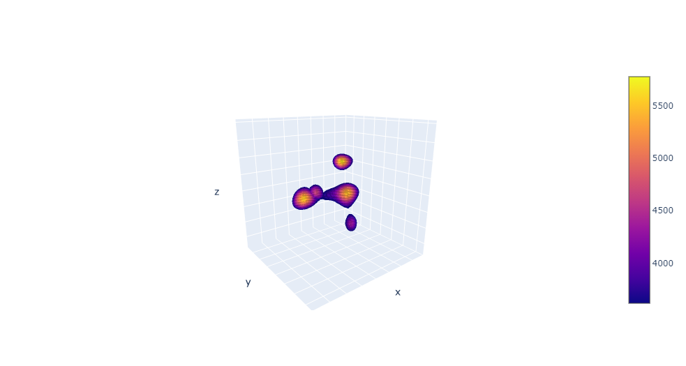
self.density_projection_3D
Use PCA 3D to project the dataset and make a 3D meshgrid to estimate the density on it with the 3D Gaussian distribution. Args:
- percentile : percentile of density that corresponds to the minimum value to show
- return_grid :If True, return 3D Grid
- return_clusters_density : If True, return the 3D Grid with the A values for each cluster
CC.density_projection_3D(99, return_grid=True, return_clusters_density=True)
{'A-Grid': array([[[3.48581797e-15, 1.62080230e-14, 6.90041904e-14, ...,
          5.83374041e-13, 1.92066889e-13, 5.70629214e-14],
         [6.60425258e-16, 6.17767595e-15, 5.01029852e-14, ...,
          3.52400611e-12, 5.50927146e-13, 7.45284376e-14]]]),
 'Clusters Density': {0: array([[[3.40385502e-48, 3.36307101e-47, 2.87017113e-46, ...,
           6.07579853e-65, 1.97018960e-66, 5.51854095e-68],
          [6.12214966e-32, 7.73521170e-31, 8.44230524e-30, ...,
           6.56667612e-49, 8.52648274e-51, 9.59653245e-53]],
         [[1.30566741e-19, 7.34944932e-19, 3.57377188e-18, ...,
           3.11782459e-28, 1.14260012e-29, 3.68476733e-31],
          [6.32366666e-22, 6.00865462e-21, 4.93929478e-20, ...,
           4.28020934e-27, 2.75837798e-28, 1.53709049e-29]]]),
  1: array([[[8.98310922e-30, 6.71213878e-29, 5.03213279e-28, ...,
           2.87124806e-29, 8.73589680e-30, 2.29930435e-30]
          [5.02339294e-21, 2.49290742e-20, 1.30264666e-19, ...,
           2.55638337e-14, 4.29622018e-15, 6.43949192e-16]],
          [2.83167266e-35, 8.65300585e-35, 2.28427319e-34, ...,
           8.11025209e-33, 1.61201265e-33, 2.82711740e-34]]]),
  2: array([[[1.36203887e-28, 9.67318866e-28, 5.96928017e-27, ...,
           1.54322295e-14, 5.09928476e-15, 1.48590282e-15],
                              ...
  8: array([[[6.84981203e-33, 1.26631274e-31, 2.37110234e-30, ...,
           9.64415278e-27, 5.73382414e-28, 3.22330467e-29],
          [1.74336209e-34, 9.68068937e-34, 4.64782487e-33, ...,
           1.05223775e-37, 1.79602795e-38, 2.64802829e-39]]]),
  9: array([[[3.60638003e-23, 1.23523984e-22, 5.16583215e-22, ...,
           5.75818352e-33, 1.73152931e-34, 4.49760341e-36],
           2.86151947e-52, 3.19445757e-53, 3.40743714e-54]]])},
 '3D Grid': {'X': array([[[-37.40388626, -37.40388626, -37.40388626, ..., -37.40388626,
           -37.40388626, -37.40388626],
          [ 38.04015058,  38.04015058,  38.04015058, ...,  38.04015058,
            38.04015058,  38.04015058]]]),
  'Y': array([[[-32.99333756, -32.99333756, -32.99333756, ..., -32.99333756,
           -32.99333756, -32.99333756],
            36.11064515,  36.11064515]]]),
  'Z': array([[[-35.1620997 , -33.64347275, -32.12484579, ...,  36.21336725,
            37.73199421,  39.25062116],
          [-35.1620997 , -33.64347275, -32.12484579, ...,  36.21336725,
            37.73199421,  39.25062116]]])}}
Utils
This section uses other modules to apply to the current self object. For example, PCA from scikit-learn is implemented. We also use UMAP from umap-learn. The list for utils methods :
- self.utils_KernelDensity - https://scikit-learn.org/stable/modules/generated/sklearn.neighbors.KernelDensity.html#sklearn.neighbors.KernelDensity
- self.utils_PCA - https://scikit-learn.org/stable/modules/generated/sklearn.decomposition.PCA.html?highlight=pca#sklearn.decomposition.PCA
- self.utils_ts_filtering_STL - https://www.statsmodels.org/devel/generated/statsmodels.tsa.seasonal.STL.html
- self.utils_UMAP - https://umap-learn.readthedocs.io/en/latest/
Graphs
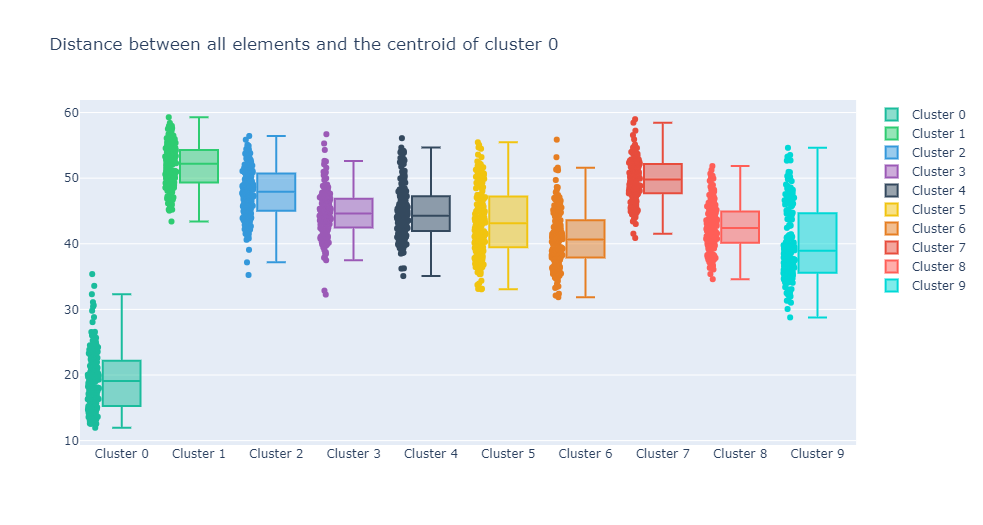
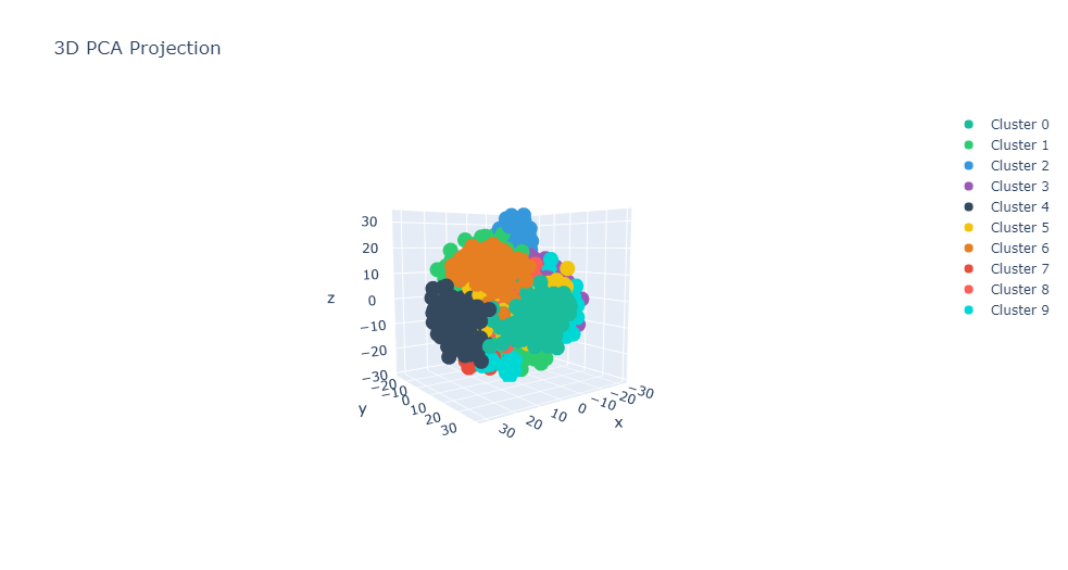
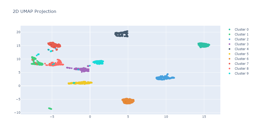
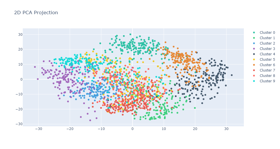
This subsclass uses Plotly to plot to different data computed with the module.
CC.graph_boxplots_distances_to_centroid(0)
CC.graph_PCA_3D()
CC.graph_reduction_2D("UMAP")
CC.graph_reduction_2D("PCA")
CC.graph_reduction_density_2D("PCA", 99, "contour")
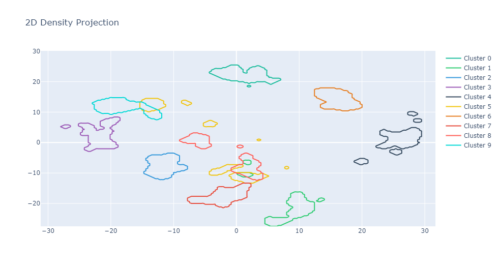
CC.graph_reduction_density_2D("UMAP", 99, "contour")
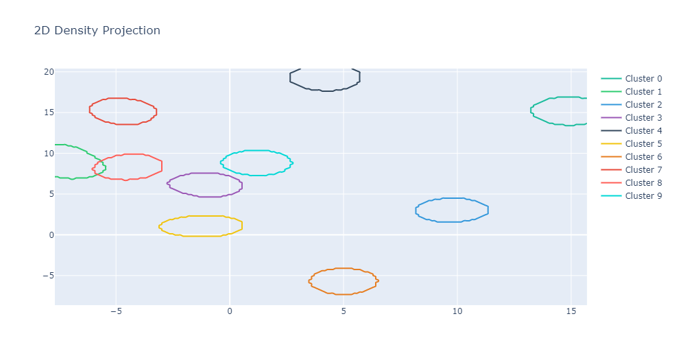
CC.graph_reduction_density_2D("PCA", 99, "interactive")
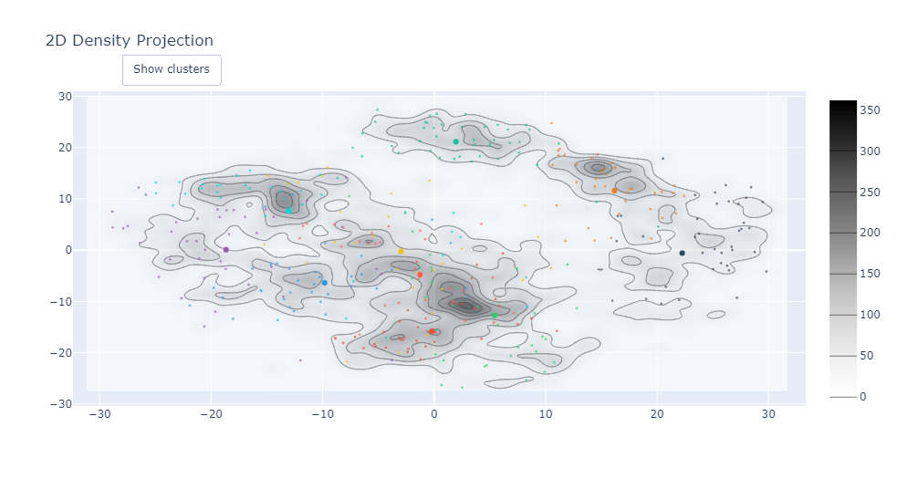
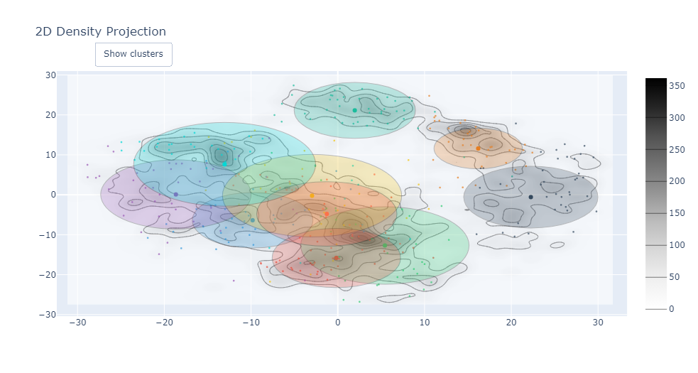
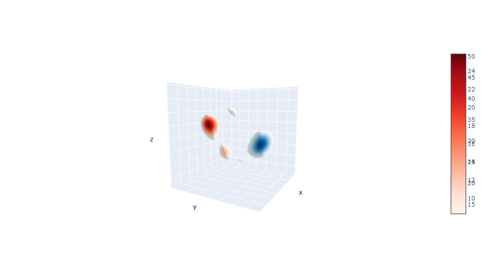
CC.graph_reduction_density_3D(99)
CC.graph_reduction_density_3D(99,clusters=[0,1])
Release history Release notifications | RSS feed


Download files
Download the file for your platform. If you're not sure which to choose, learn more about installing packages.
Source Distributions
Built Distribution
Filter files by name, interpreter, ABI, and platform.
If you're not sure about the file name format, learn more about wheel file names.
Copy a direct link to the current filters
File details
Details for the file Clusters_Features-1.0.3-py3-none-any.whl.
File metadata
- Download URL: Clusters_Features-1.0.3-py3-none-any.whl
- Upload date:
- Size: 65.6 kB
- Tags: Python 3
- Uploaded using Trusted Publishing? No
- Uploaded via: twine/3.4.2 importlib_metadata/4.7.1 pkginfo/1.7.1 requests/2.26.0 requests-toolbelt/0.9.1 tqdm/4.62.2 CPython/3.7.11
File hashes
| Algorithm | Hash digest | |
|---|---|---|
| SHA256 |
6fea31627a763385feee9368f8dcaeaf0499d872131946094abceef5d3b19663
|
|
| MD5 |
3c7e5895fcc4d1794fabc8e6a5d3e9de
|
|
| BLAKE2b-256 |
84538f4f615a1505728785d76cff090f0558607257d006b9ff2fc53e54ef2e9e
|


