




DaSPi — Process Analytics & Six Sigma in Python
DaSPi helps engineers analyze and improve processes using statistical workflows.
🎯 The Problem
Process analysis in practice is fragmented:
- Excel is error-prone and hard to scale
- Minitab / JMP are expensive and closed
- Python tools (pandas, scipy, statsmodels) are powerful but disconnected
👉 Engineers spend more time combining tools than improving processes.
✅ The Solution
DaSPi provides integrated workflows for process analytics:
- Capability analysis (Cp, Cpk)
- Root cause analysis (ANOVA, regression)
- Statistical process control (SPC)
- Professional visualization
All in one consistent and intuitive interface.
🚀 Four Flagship Workflows
DaSPi provides four ready-to-use workflows that cover the complete quality cycle. Each workflow produces visual output + interpretation in under 20 lines of code.
📏 Workflow 1: Gage R&R Analysis
Verify your measurement system is capable before analyzing process data.
import daspi as dsp

# Load data
df = dsp.load_dataset("grnr_layer_thickness")

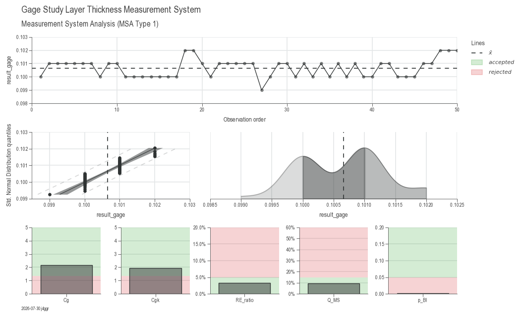
# Step 1: Evaluate the gage itself (MSA Type 1)
gage = dsp.GageStudyModel(
    source=df,
    target="result_gage",
    reference="reference",
    u_cal=df["U_cal"][0],
    tolerance=df["tolerance"][0],
    resolution=df["resolution"][0]
)

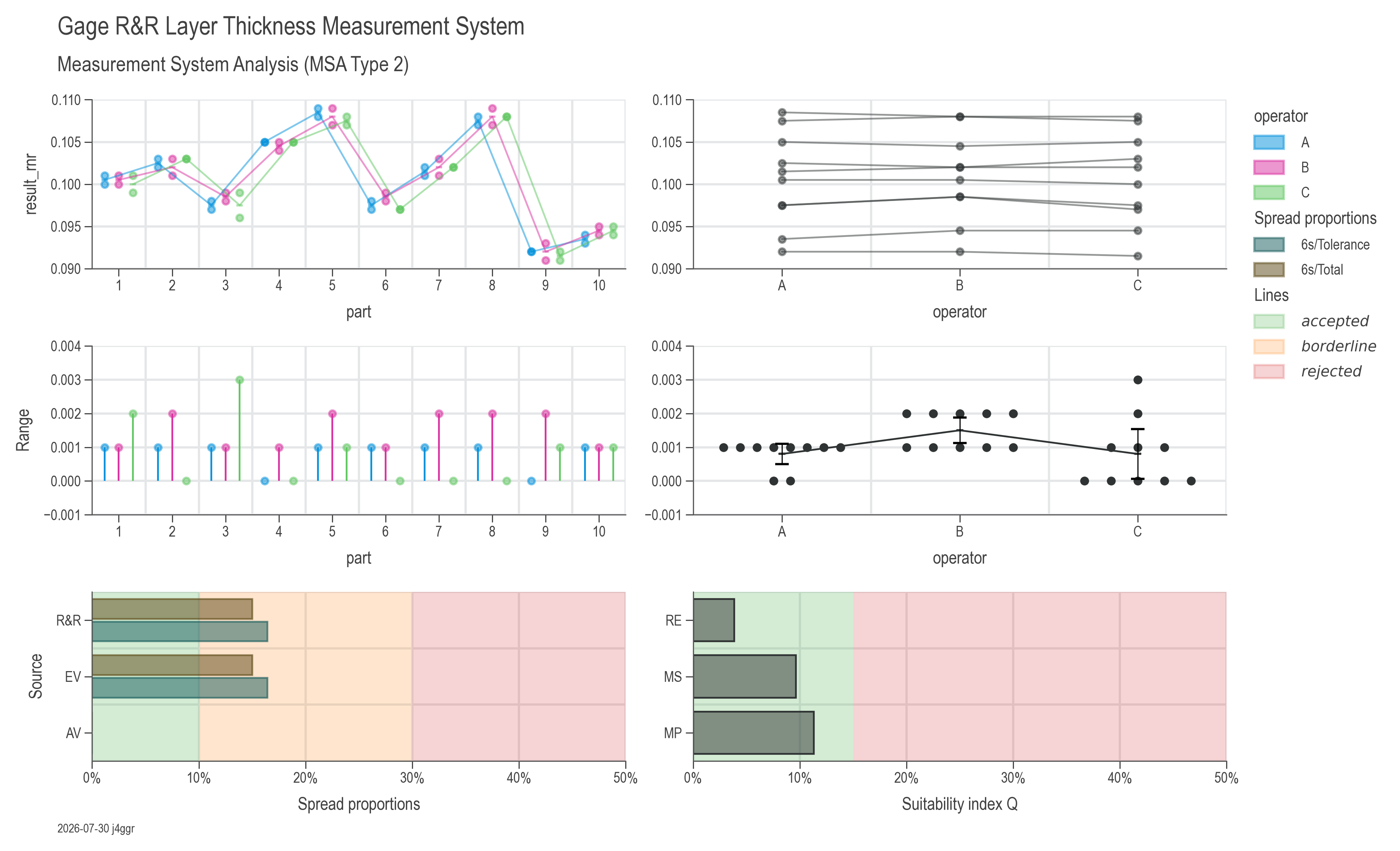
# Step 2: Evaluate repeatability & reproducibility (MSA Type 2)
model = dsp.GageRnRModel(
    source=df,
    target="result_rnr",
    part="part",
    gage=gage,
    u_av="operator"  # Operator variation
)

# Step 3: Visualize complete analysis
chart_gage = dsp.GageStudyCharts(
        gage,
        stretch_figsize=1.5
    ).plot(
    ).stripes(
    ).label(
        fig_title='Gage Study Layer Thickness Measurement System',
        sub_title='Measurement System Analysis (MSA Type 1)',
        info=True)

chart_rnr = dsp.GageRnRCharts(
        model,
        spread_accepted_limit=0.1,   # 10% threshold for acceptance
        spread_rejected_limit=0.3,   # 30% threshold for rejection
        u_accepted_limit=0.15,       # 15% uncertainty threshold
        stretch_figsize=1.5
    ).plot(
    ).stripes(  # Adds acceptance zones
    ).label(
        fig_title='Gage R&R Layer Thickness Measurement System',
        sub_title='Measurement System Analysis (MSA Type 2)',
        info=True)
Output: Comprehensive measurement system evaluation with repeatability (EV), reproducibility (AV), variance components, ANOVA tables, and capability indices (Cg, Cgk).
📊 Workflow 2: Process Capability Analysis
Evaluate if your process meets specifications.
import daspi as dsp

# Load data
df = dsp.load_dataset("drop_card")
spec_limits = dsp.SpecLimits(0, float(df.loc[0, "usl"]))

# Analyze capability
chart = dsp.ProcessCapabilityAnalysisCharts(
    source=df,
    target="distance",
    spec_limits=spec_limits,
    hue="method"
).plot().stripes().label(
    fig_title="Process Capability Analysis of Drop Card Data",
    sub_title="Drop Card Distance Comparison between Two Methods",
    target_label="Distance s (cm)",
    info=True)

chart.show()
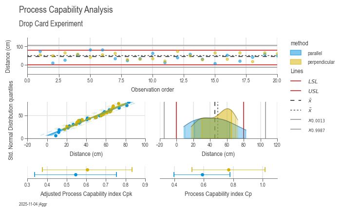
Output: 5-panel analysis with Cp, Cpk, Pp, Ppk, distribution plots, and statistical interpretation.
🔍 Workflow 3: Root Cause Analysis
Identify which factors significantly impact your process.
import daspi as dsp

# Load data
df = dsp.load_dataset("painkillers-dissolution")

# Fit model with automatic factor selection
model = dsp.LinearModel(
    source=df,
    target="dissolution",
    factors=["employee", "brand", "water", "catalyst"],
    covariates=["temperature"],
    order=2,
)

# Perform recursive elimination to select significant factors
df_gof = pd.concat(model.recursive_elimination())

# Visualize results
chart_res = dsp.ResidualsCharts(model).plot().stripes().label(info=True)
chart_param = dsp.ParameterRelevanceCharts(model).plot().stripes().label(info=True)
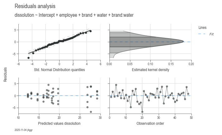
Output: Residual diagnostics + parameter effects with ANOVA tables and significance tests.
📈 Workflow 4: Statistical Process Control (SPC)
Monitor process stability and detect out-of-control conditions.
import daspi as dsp

# Load process data
df = dsp.load_dataset("grnr_spc")

# Create control chart
chart = dsp.JointChart(
        source=df,
        target='result',
        feature=('measurement_order', ''),
        nrows=1,
        ncols=2,
        width_ratios=[4, 1],
        sharey=True,
    ).plot(
        dsp.Scatter
    ).plot(
        dsp.Line,
        on_last_axes=True,
    ).plot(
        dsp.GaussianKDE,
        hide_axis='feature',
        visible_spines='target',
    ).stripes(
        mean=True,
        control_limits=True,    # UCL/LCL at 3-sigma
        agreement=3,            # 3-sigma agreement lines
        strategy='norm',        # Use normal distribution for control limits
    ).label(
        fig_title='SPC Chart: Layer Thickness',
        sub_title='Control limits at ±3σ',
        target_label='Layer Thickness (µm)',
        feature_label=('Measurement Order', ''),
        info=True
    )

chart.show()
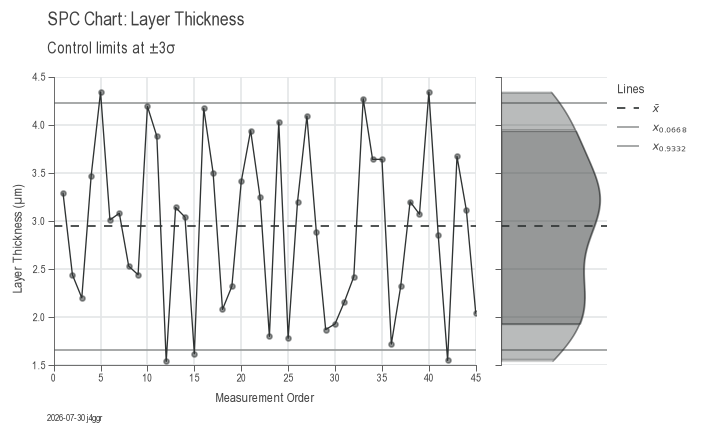
Output: Control chart with mean, control limits (UCL/LCL), specification limits, and trend analysis.
🏭 Use Cases
- Manufacturing: Monitor tolerances and reduce defects
- Quality Engineering: Automate Six Sigma DMAIC workflows
- Process Optimization: Identify key drivers of variation
- Data Analysts: Unify statistics and visualization in one tool
📊 Example Outputs
MSA1: Gage Study (Single Reference)
MSA2: Gage R&R (Repeatability & Reproducibility)
Process Capability Analysis
Root Cause Analysis (ANOVA)
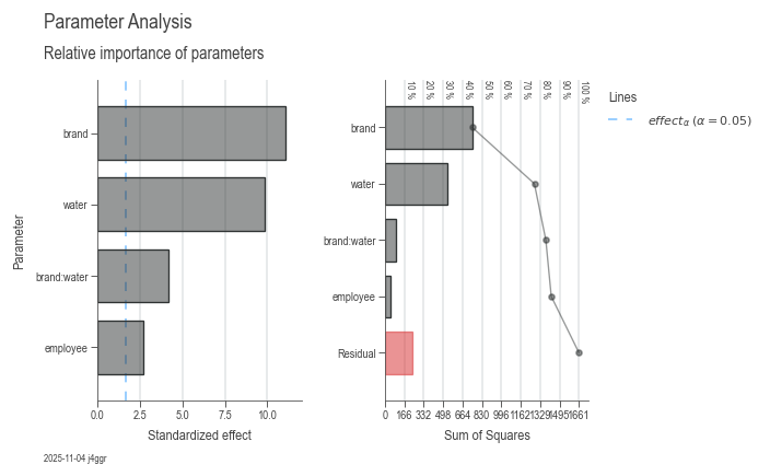
formula:
dissolution ~ 26.8292 + 2.3750employee[T.B] + 0.8375employee[T.C] - 10.7500brand[T.ZapPain] - 9.5167water[T.tap] + 5.7167*brand[T.ZapPain]:water[T.tap]
Model Summary:
| hierarchical | least_parameter | p_least | s | aic | r2 | r2_adj | r2_pred | |
|---|---|---|---|---|---|---|---|---|
| 0 | True | employee | 0.023298 | 2.374693 | 224.835935 | 0.857379 | 0.840400 | 0.813719 |
Parameter statistics:
| coef | std err | t | p | ci_low | ci_upp | |
|---|---|---|---|---|---|---|
| Intercept | 26.829167 | 0.839581 | 31.955433 | 0.000000 | 25.134824 | 28.523509 |
| employee[T.B] | 2.375000 | 0.839581 | 2.828793 | 0.007133 | 0.680657 | 4.069343 |
| employee[T.C] | 0.837500 | 0.839581 | 0.997522 | 0.324224 | -0.856843 | 2.531843 |
| brand[T.ZapPain] | -10.750000 | 0.969464 | -11.088598 | 0.000000 | -12.706458 | -8.793542 |
| water[T.tap] | -9.516667 | 0.969464 | -9.816417 | 0.000000 | -11.473125 | -7.560208 |
| brand[T.ZapPain]:water[T.tap] | 5.716667 | 1.371030 | 4.169616 | 0.000149 | 2.949817 | 8.483516 |
Analysis of variance:
| Typ-I | DF | SS | MS | F | p | n2 |
|---|---|---|---|---|---|---|
| employee | 2 | 46.431667 | 23.215833 | 4.116891 | 0.023298 | 0.027960 |
| brand | 1 | 747.340833 | 747.340833 | 132.526821 | 0.000000 | 0.450027 |
| water | 1 | 532.000833 | 532.000833 | 94.340328 | 0.000000 | 0.320355 |
| brand:water | 1 | 98.040833 | 98.040833 | 17.385695 | 0.000149 | 0.059037 |
| Residual | 42 | 236.845000 | 5.639167 | nan | nan | 0.142621 |
Variance inflation factor:
| DF | VIF | GVIF | Threshold | Collinear | Method | |
|---|---|---|---|---|---|---|
| Intercept | 1 | 5.000000 | 2.236068 | 2.236068 | True | R_squared |
| employee | 2 | 1.000000 | 1.000000 | 1.495349 | False | generalized |
| brand | 1 | 1.000000 | 1.000000 | 2.236068 | False | R_squared |
| water | 1 | 1.000000 | 1.000000 | 2.236068 | False | R_squared |
| brand:water | 1 | 1.000000 | 1.000000 | 2.236068 | False | single_order-2_term |
SPC: Control Chart with Mean, UCL/LCL, Specification Limits
🚀 Installation
pip install daspi
📚 Documentation
- User Guide — Complete tutorials for each workflow
- API Reference — Detailed documentation
- 3S Methodology — Structured problem-solving
🔧 Technical Features
- Centralized configuration — Manage language, username, and styles globally
- Multivariate visualization — Explore complex relationships
- Linear models & ANOVA — Statistical inference made simple
- Hypothesis testing — Confidence intervals and p-values
- Monte Carlo simulation — Assess uncertainty
- Process capability — Cp, Cpk, Pp, Ppk calculations
⚙️ Built on Proven Libraries
DaSPi leverages the Python scientific stack:
- pandas — Data manipulation
- numpy — Numerical computing
- matplotlib — Visualization
- scipy — Statistical functions
- statsmodels — Advanced statistics
👤 About
DaSPi is created and maintained by Reto Jäggli, Data Scientist at Festo Microtechnology AG.
The project is driven by a passion to make process analytics and Six Sigma workflows more accessible in Python.
⚠️ Disclaimer
DaSPi is under active development and may contain bugs.
Results should be validated with trusted statistical tools when required.
🤝 Feedback & Contributions
If you use DaSPi in real-world process analysis:
👉 I would love to hear your use case.
Feedback, ideas, and contributions are very welcome.
1 maintainer

Metadata
1 maintainer
Release files for DaSPi 2.2.0
For a detailed explanation of source distributions (sdists) and built distributions (wheels), please see the package formats documentation.
Source distribution (sdist)
| File | Size | Uploaded | |
|---|---|---|---|
| daspi-2.2.0.tar.gz | 17.0 MB | Details |
Built distribution (wheel)
| File | Interpreter | ABI | Platform | Reset |
|---|---|---|---|---|
| daspi-2.2.0-py3-none-any.whl | Python 3 | none | any | Details |
Total release size: 17.4 MB
Release files / daspi-2.2.0.tar.gz
| Download URL | daspi-2.2.0.tar.gz |
|---|---|
| Size | 17.0 MB |
| Tags | Source |
|
SHA-256 checksum How to use checksums |
95b835bcb53bdd381d996f5e522e8020e195577e866a6072c0a65694dd549c52
|
|
BLAKE2b-256 checksum How to use checksums |
b779fa590d3e5d847450ec69cfb355ec94f52c35d176a2b9b89d1273ea0608c5
|
| Upload date | |
|
Uploaded using Trusted Publishing? What is trusted publishing? |
No |
| Uploaded via |
pdm/2.28.0 CPython/3.12.3 Windows/11
|
Release files / daspi-2.2.0-py3-none-any.whl
| Download URL | daspi-2.2.0-py3-none-any.whl |
|---|---|
| Size | 375.1 kB |
| Tags | Python 3 |
|
SHA-256 checksum How to use checksums |
4f97f8a1473676b0c4c17a5a0e1a509bf76908ef085d5d9e308e3315ff176eef
|
|
BLAKE2b-256 checksum How to use checksums |
1741786bc7520f682767673f64b72e5276cffa9853af2036df9456a5f3959f13
|
| Upload date | |
|
Uploaded using Trusted Publishing? What is trusted publishing? |
No |
| Uploaded via |
pdm/2.28.0 CPython/3.12.3 Windows/11
|














