
betula-cluster







Rust-powered, memory-bounded clustering for large embeddings & tabular streams. It compresses raw data into numerically stable BETULA microclusters, then runs the clustering head on the compressed representation — k-means · GMM (diagonal & full) · Ward · spectral · Leiden community detection · directional (von Mises–Fisher / spherical) · HDBSCAN-CF · scale-space modes · Mapper — so cost scales with the microcluster count, not
N. Streamingpartial_fit, a scikit-learn API, from-scratch Rust core + PyO3, no LAPACK or SciPy at runtime.
pip install betula-cluster
Verified: a 457-case Python suite at 100% wrapper coverage + 728 Rust tests,
clippy -D warnings + fmt clean across all feature sets, CI on CPython 3.11–3.14 (one abi3 wheel).
At a glance — honest benchmarks
Measured against scikit-learn on StandardScaler-normalized data, each method in its own subprocess
with peak RSS sampled from /proc/self/statm. Full methodology, every metric, and all tables (wins
and losses) live in bench/RESULTS.md.
Re-measured 2026-09-07 against the 0.8.0 tree, on a machine gated to be idle. Every quality figure is the median of seeds 0, 1, 2 — clustering quality is seed-dependent and a single run is not a result. Ranges per cell are in
bench/results_*_spread.csv; on the synthetic sets every row moves by more than 0.05 ARI across the three seeds, so a margin below that is a tie and is written as one here.
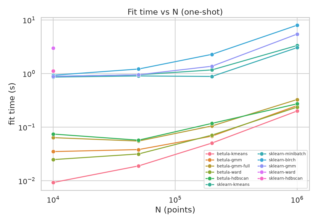
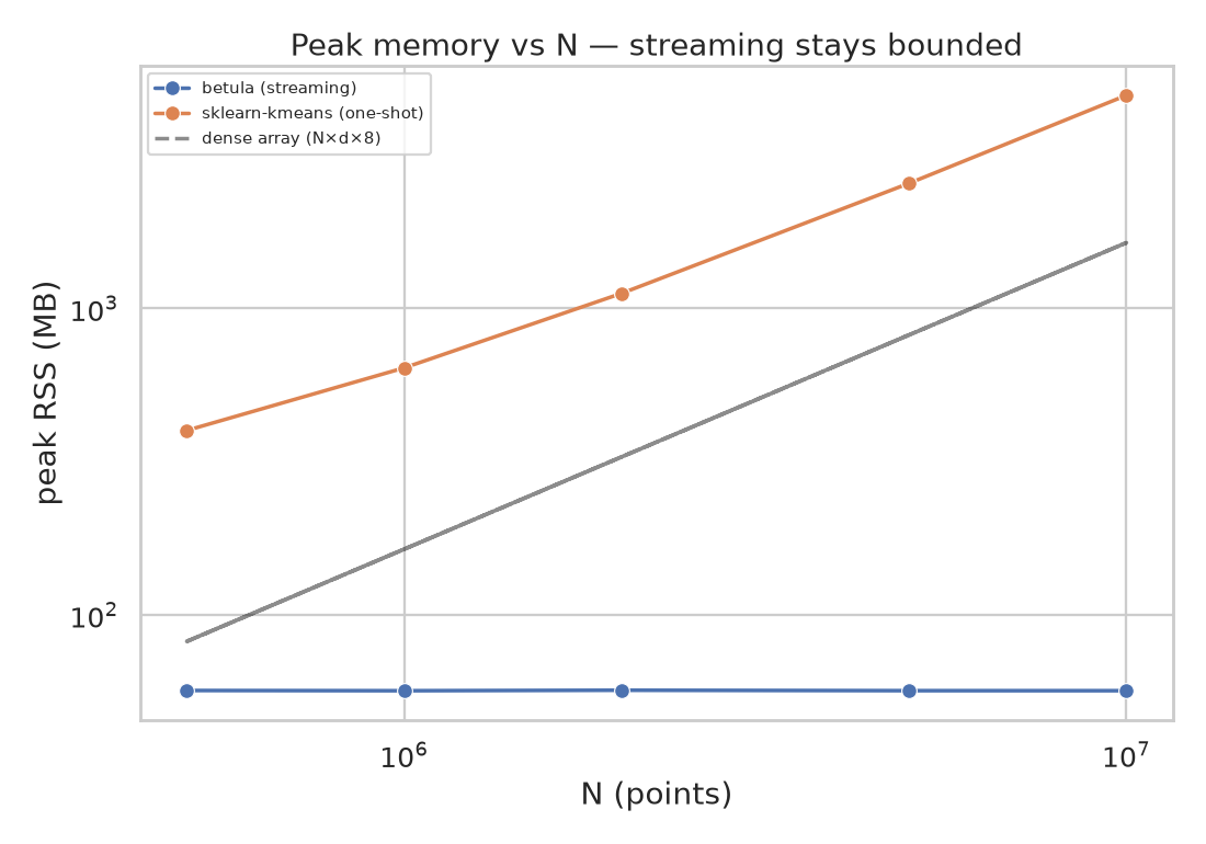
- ⚡🪶 Always faster — and lighter — at scale (the unconditional win). betula labels 1 M points in 0.28 s: 8.7× faster than scikit-learn KMeans, 14× vs GaussianMixture, 29× vs Birch — and streams 10 M in a flat ~53 MB where an in-core KMeans needs ~5.0 GB (94× less, and the gap grows without bound). This holds for every method at every size.
- 🎯 Parity on the centroid heads, ahead on the structured ones. betula's k-means ties
scikit-learn (blobs 0.793 vs 0.794,
digits0.467 vs 0.468); full-covariance GMM beats it on anisotropic data (0.961 vs 0.902) and on real 64-Ddigits(0.575 vs 0.463, via the high-dimensional covariance floor); betula-ward clusters 1 M in 0.42 s whereO(N²)sklearn-ward can't run past ~10 k; and on non-convex moons & circles the spectral and HDBSCAN heads hit ARI 1.00. Spectral matchesSpectralClustering's quality; the speed ratio is not worth quoting — it has read 3–5×, 1.0–1.5× and 2.4–2.5× across editions and the movement is in scikit-learn's arm, not ours. The durable claim is scaling: cost set bymax_leaves, notN. - 🌍 Real data, and two losses stated plainly. betula's diagonal GMM overtakes scikit-learn on hard
covtype(0.104 vs 0.080 at adequate leaf resolution — at the default 4 000-leaf budget the two are a tie inside their seed spreads) and it clusters full covtype (581 k rows) 5.5× faster at no worse ARI (0.070 vs 0.049). Butsklearn-birchbeats every betula head on bothcovtype(0.131) and MNIST (0.426 vs 0.377). Oncovtypethat is a loss on the merits — tested in both directions, and the mechanism is the leaf budget's unequal cell mass; on MNIST Birch simply does not compress (20 000 subclusters for 20 000 points), and at equal compression the gap falls from 0.059 to 0.010. HDBSCAN-on-CF likewise trails raw HDBSCAN on overlapping density.bench/RESULTS.mdreports both rather than hiding them.
 |
 |
|---|---|
| Phase-3 clusters only the ~2 000 leaf microclusters, not the raw points, so every head finishes 1 M points in under 0.55 s (k-means in 0.28 s). | The CF-tree is capped by max_leaves, so streaming memory stays flat — it clusters data larger than RAM. |
Why
Who it's for: practitioners clustering large embedding or tabular datasets — in batch or as a stream — who need bounded memory and the numerical stability that classic BIRCH and in-core scikit-learn don't provide together.
Clustering libraries tend to either not scale (full GMM/HDBSCAN on raw points), lose precision
(classic BIRCH computes variance as SS − ‖LS‖²/n, which catastrophically cancels far from the
origin), or blow up in memory (BIRCH-family subcluster explosion in high dimensions). betula-cluster
addresses all three:
- Numerically stable — clustering features
(n, μ, S)via Welford / Chan updates; the covariance is PSD by construction. Classic BIRCH loses all digits near coordinate1e7; betula does not. - Memory-bounded by design — the CF-tree caps its leaves (
max_leaves) and rebuilds, so it never explodes; streaming memory is flat inNand clusters data larger than RAM. - Complete — one stable engine spanning k-means / GMM (diag & full) / Ward / spectral / Leiden
community detection / HDBSCAN-style / Mapper, with streaming
partial_fit, a scikit-learn API, and dataset-structure inspection.
The math (stable CF, the expected-log GMM E-step, distance derivations, relation to BIRCH/BETULA) is
written up — verified symbolically and numerically — in docs/MATH.md.
When to use it
Reach for betula-cluster when the data is large or streaming, memory must stay bounded, you want
fast predict on new points, or you want one numerically stable engine spanning k-means / GMM / Ward /
density / topology plus dedup / outliers / representatives — especially on embeddings and tabular
streams.
Use raw scikit-learn instead when N fits comfortably in RAM and you want the exact point-level
algorithm with no compression: at small N the two-phase overhead removes the speed edge, and raw
HDBSCAN is stronger on overlapping density. betula-cluster trades a CF-compression approximation for
scale and bounded memory — if you need neither, a plain in-core clusterer is simpler.
Installation
pip install betula-cluster            # prebuilt abi3 wheels, CPython 3.11–3.14
pip install 'betula-cluster[tune]'    # + Optuna backend for memory-aware tuning
NumPy is the only runtime dependency — no SciPy, LAPACK, or BLAS. Prebuilt wheels ship for Linux
(x86-64 + aarch64), macOS (Intel + Apple Silicon), and Windows (x64); one abi3 wheel covers every
supported Python. Building from source needs a Rust toolchain — maturin develop --release (or
pip install .) in a clone.
Quick start
import numpy as np
import betula_cluster

X = np.random.default_rng(0).normal(size=(100_000, 10))

labels = betula_cluster.fit_predict(X, n_clusters=10, method="kmeans")
labels = betula_cluster.fit_predict(X, n_clusters=0, feature="full", method="gmm-full")  # auto-k via BIC
labels = betula_cluster.fit_predict(X, n_clusters=8, method="spectral", threshold=0.0)   # non-convex / manifold
labels = betula_cluster.fit_predict(X, method="leiden", threshold=0.4)                    # graph communities; count auto-discovered
labels = betula_cluster.fit_predict(X, method="hdbscan", min_cluster_size=25)            # HDBSCAN-CF; -1 = noise
labels = betula_cluster.fit_predict(X, n_clusters=10, method="vmf")                       # directional / cosine (input auto-L2-normalized)
labels = betula_cluster.fit_predict(X, n_clusters=4, method="watson", feature="full")     # axial: x and -x are the same point
Streaming / out-of-core — feed chunks, finalize, predict; memory stays bounded by max_leaves:
est = betula_cluster.Betula(method="gmm", memory_budget_mb=512)
for chunk in stream_of_arrays:        # each chunk is a 2-D float32/float64 array
    est.partial_fit(chunk)
est.partial_fit()                     # finalize the global clustering over everything seen
labels = est.predict(X_query)
Reproducibility — every BIRCH-family tree builds its prototype set as a greedy threshold-net in
arrival order, so the same rows in a different order give a different answer; at real compression
that matters more than the seed does (order pairwise ARI 0.55 against the seed arm's 0.75, over 27
measured cells). canonical_order=True sorts the rows by a key derived from the data before the
first insert, which makes the summary a function of the multiset — and the guarantee is exact:
labels_a = betula_cluster.fit_predict(X, 10, canonical_order=True)
labels_b = betula_cluster.fit_predict(X[perm], 10, canonical_order=True)
assert (labels_a == labels_b[np.argsort(perm)]).all()   # equal element for element, in all 27 cells
It buys reproducibility, not accuracy — the median quality change is −0.002 ARI, and the realised
leaf count stops varying too. Numbers, costs and the two cells where it loses:
bench/RESULTS.md.
Robustness — with the default arrival order, consensus clusters several random permutations and
votes, returning a consensus labelling plus a per-point stability score (any partitional head —
kmeans / gmm / ward / spectral):
res = betula_cluster.consensus(X, n_clusters=10, n_runs=5, method="kmeans", n_jobs=-1)  # -1 = all cores
res.labels           # (n,) consensus label per point
res.confidence       # (n,) in [0, 1] — per-point agreement across runs (1.0 = every order agrees)
res.mean_confidence  # scalar robustness summary
Memory-aware hyperparameter tuning (tune, optional Optuna), Mapper topology (mapper),
semi-supervised constraints (COP-KMeans), mixed numeric+categorical+directional (KPrototypes),
streaming density (DenStream / DbStream), the O(nnz) sparse-native path (fit_predict_sparse),
CF-weighted NMF for nonnegative data (projection="weighted-nmf", or "weighted-nmf-kl" for counts),
quantile
sketches, scipy.sparse input, threshold="auto", soft assignment / coresets / diagnostics / drift
snapshots / active-learning batches, the Rust API, and the CLI — all in the
usage guide.
Capabilities
Stable core — production-ready:
- Clustering heads — weighted k-means (Hamerly), GMM (diagonal & full covariance, BIC auto-
k), exact Ward HAC, spectral (non-convex / manifold), Leiden graph community detection (auto community count,resolution/ CPM, optional covariance/manifold-aware affinity), and directional spherical k-means / von Mises–Fisher mixtures for L2-normalized embeddings (cosine geometry), all over the numerically stable BETULA CF-tree. - Streaming —
partial_fitat bounded memory (max_leaves/memory_budget_mb), EWMAdecay. - scikit-learn API —
fit/predict/fit_predict,get_params/set_params(works withPipeline/clone/GridSearchCV); typed abi3 wheel,save/load+ pickle, reusable Rust core. - Inspection & robustness —
predict_proba, coresets, microcluster/cluster geometry, outliers, near-duplicates, representatives, diagnostics, andconsensus(per-point stability across insertion-order permutations). - Order-invariant builds —
canonical_order=Truemakes the summary a function of the multiset, so any row permutation returns bit-identical labels. Measured exact in all 27 cells of the published sweep; no other BIRCH-family implementation publishes such a guarantee. - Tuning —
tune: memory-aware hyperparameter search with a quality / memory / speed Pareto mode; NumPy-only, optional Optuna backend (pip install 'betula-cluster[tune]').
Experimental / evolving — useful today, API may still move:
- Density & topology — HDBSCAN-CF (density over microclusters), scale-space Morse-persistence
density-mode clustering (
method="scale-space"— nok, no bandwidth), and a Mapper topological skeleton (mapper/mapper_stability). - Naming
kon the density hierarchy (method="dc-median"/"dc-center", Beer et al. 2023) — exactk-median /k-center in the density-connectivity ultrametric, cutting the same mutual-reachability treehdbscanreads its count off.dc-medianbeatsspectralby 0.198 on noisy moons at 20× less wall clock and tieswardondigits;dc-centeris mass-blind by construction and is published with the measurement that shows it. - OPTICS reachability plot (
reachability()→ReachabilityPlot) — the density diagnostic, over the microclusters. Not a lookalike ofmethod="hdbscan": OPTICS with no ε cutoff is Prim on the mutual-reachability graph, so the sweep walks that head's own spanning tree andlabels_at(ε)is its hierarchy cut at ε, exactly. Cost is set by the leaf count, not byN— 0.0028 s at both 20 000 and 320 000 rows. - X-means (
method="xmeans", Pelleg & Moore 2000) — recursive splitting instead of aksweep:n_clustersis an upper bound rather than a target, and it is the only auto-khead that can return more than 20 clusters. Its split test needs a cut capturing1 − 2^(−2/d)of a region's scatter, so it lands on the true count at everyd ≥ 5and under-splits only atd = 2— see Wherexmeansrefuses to split. - k-medoids (
method="kmedoids", eager FasterPAM — Schubert & Rousseeuw 2021) — the centre of a cluster is one of the summary's own micro-clusters rather than an average: an exemplar you can show, and a centre that stays on the data manifold. Exact on the summary, becauseΣ_{x∈leaf} ‖x − μ‖² = S + n‖μ_leaf − μ‖²makes the leaf-level objective the point-level one — note the square, since classical PAM's absolute distance has no closed form in a cluster feature. Ondigitsat one leaf per point it reads ARI 0.554 [0.554–0.570] againstkmeans's 0.467 [0.443–0.571] over seeds 0–4, and loses at a coarse summary (115 leaves: 0.219 vs 0.240) where there are too few candidate centres; theO(m²)swap pass costs 6×kmeansat 1797 leaves.n_clusters=0switches objective to the medoid silhouette, because total deviation is monotone ink—docs/USAGE.md. - Fuzzy c-means (
method="fuzzy-cmeans", Bezdek 1981) — the only soft head that fits no density: it publishes a partition of unityu_j ∝ d_j^(−1/(m−1))over the centres, exact on the summary by the same identitykmedoidsuses, with Xie–Beni as its automatick. Take it for the membership, not for the labels — the hard partition is a loss againstkmeanson every fixture measured (blobs0.847 vs 0.864,aniso0.535 vs 0.545,digits0.483 vs 0.467 atm=1.3), and the loss grows with cluster overlap and withm, because no membership is ever zero and every centre is pulled toward the grand mean —docs/USAGE.md. - Structured-covariance GMM — a three-rung Toeplitz ladder:
method="gmm-toeplitz"(banded AR),"gmm-toeplitz-full"(general positive-definite Toeplitz covariance), and"gmm-toeplitz-gs"(full-order Gohberg–Semencul MLE precision): covariance-shape clustering for ordered, stationary signals (time-series windows, trajectories, sensor waveforms), well-posed where full covariance is singular (N_k ≪ d) and a diagonal model ignores neighbour correlation; the-fullhead captures structure beyond a low-order AR (e.g. a long-lag echo), the-gshead fits a likelihood-optimal precision with a cheaper E-step than full at larged. - Subspace GMM —
method="mppca", a mixture of probabilistic PCA (Tipping & Bishop 1999): each component covariance isW Wᵀ + σ²Iof rankrank, so it carries orientation atO(d·rank)per component instead ofO(d²)and runs atd = 784where the full head cannot. At one leaf per point ondigitsit beats both the diagonal and the full head (ARI 0.600 vs 0.461 / 0.575); on a coarse summary it loses to the diagonal head, anddocs/USAGE.mdmeasures why. - Factor-analyser GMM —
method="mfa"(Ghahramani & Hinton 1996), the same subspace model withmppca's singleσ²relaxed to a per-dimensiondiag(ψ), for tables whose columns are in different units and cannot be standardised. The two heads dissociate in both directions on controlled fixtures —mfareads a quiet axis that a loud nuisance pair drowns (ARI 1.00 vsmppca's 0.04–0.34),mppcareads lines that differ only in orientation (1.00 vs ≈ 0.00) — but on real tables already on a common scalemppcawins every row measured (digits0.738 vs 0.562, MNIST-20k 0.365 vs 0.277). Whatmfabuys is a floor, not a ceiling: it contains the diagonal Gaussian mixture atrank=0and falls back onto it, wheremppcacan land at less than half its score. Not rotation-equivariant, for the same reasongmmis not.docs/USAGE.mdhas the tables. - Axial mixture —
method="watson"(Watson 1965), for directional data whose sign is arbitrary: eigenvectors, SVD/PCA axes, line orientations, any feature wherexand−xare the same observation.p(x) ∝ exp(κ (μᵀx)²)is antipodally symmetric, so wherevmfspends half its components on the antipodes of the other half, this reads one axis. Its sufficient statistic is the second momentΣ_i + μ_i μ_iᵀ, which thefullleaf carries exactly — the E-step is closed form, not an approximation. On a 32-D four-axis fixture with half of each cluster at each pole it scores ARI 0.953 againstvmf's 0.218 andgmm-full's 0.316, and its BIC findsk = 4wherevmfanswers 8; ondigits-PCA20 with a random half of the rows sign-flipped it moves 0.498 → 0.503 while every other head loses 60–70 %. The trade is explicit: where the sign does carry information it loses tovmf(0.952 vs 0.976), and it costs 5–8×vmfin wall clock.κ < 0fits girdle (equatorial) components too, andn_clusters=0selectskby BIC —docs/USAGE.md. - Hyperbolic embeddings —
method="hyperbolic"(Law et al., ICML 2019) for data that is already a point set ofH^d: Poincaré or Lorentz coordinates of a taxonomy, ontology or scale-free graph. It clusters under the squared Lorentzian distanced_L² = −2 − 2⟨x,y⟩_L, whose centroid is the normalised sumR/|R|_L— and which is affine, so a leaf enters only through(n_i, R_i)and its covariance is not read at all. That makesfeature="spherical"exactly as good as"full"(measured: identical to four digits), which is true of no other head here. The deliverable is invariance, not ARI: a Lorentz boost is an isometry ofH^d, and on a 15 360-point tree embedding boosted by rapidity 3 the Poincaré-ball route withgmm-fullfalls 0.817 → 0.311 while this head holds 0.731 → 0.596. On an un-boosted embedding that ball route wins outright, and the residual drift here is the Euclidean CF-tree's, not the head's — at one leaf per point the head is exactly boost-invariant (0.772 at every rapidity). The trade, and thef64working radius of ≈ 18, are indocs/USAGE.md. - More heads & data —
DenStream/DbStreamevolving-stream density, mergeableKllSketch/DdSketchquantiles,scipy.sparse(O(nnz), never densified), mixed numeric+categorical+directional (KPrototypes), COP-KMeans constraints, robust (Huber) insertion, drift snapshots, dependency-free CLI.
Full reference: docs/FEATURES.md.
Examples
Seventeen executed, plotted notebooks — one per capability — live in
examples/ (render on GitHub):
- Core — quickstart, embeddings & inspection, streaming & persistence, method comparison, Mapper topology.
- Streaming density —
DenStream&DbStream. - Mixed data —
KPrototypes. - Sketches —
KllSketch&DdSketch. - Semi-supervised — must-link / cannot-link.
- Sparse / high-dim —
scipy.sparse+fit_predict_sparse. - Soft assignment & coresets —
predict_proba, coresets, diagnostics. - Production ops — drift, active learning, robust, memory budgets.
- Graph & geometry — graph clustering (Leiden), directional embeddings (vMF / spherical), geometry-aware clustering (covariance / manifold).
- Time-series —
gmm-toeplitzAR/Toeplitz covariance for stationary signals. - Nonnegative data —
projection="weighted-nmf"CF-weighted NMF on topic counts.
And six end-to-end use cases (each scored against ground truth):
- 🧹 Embedding dedup — collapse a repost-heavy corpus to representatives.
- 🚨 Log anomaly detection — batch outlier scoring + streaming
DbStreamflags. - 👥 Customer segmentation — mixed RFM + categorical personas with
KPrototypes. - 🧠 RAG corpus curation — junk removal, topic coherence, and topic-leakage detection via Mapper.
- 🔢 Real-data clustering — handwritten digits, ARI parity + centroid/exemplar inspection.
- 🌐 Graph communities — Leiden community detection on a network, scored against planted communities.
Documentation
- Usage guide — runnable snippets for every interface.
- Features — full capability reference + crate architecture.
- Math — stable CF, GMM E-step, distance derivations, relation to BIRCH/BETULA.
- Benchmarks — methodology, every metric, all tables, honest wins & losses.
- Design — internal design, invariants, and testing strategy.
Verified: 713 Rust unit + 15 integration tests (plus 8 for the CLI binary) + a 457-case
Python suite at 100% wrapper coverage (Rust ≥95%, CI-enforced), clippy -D warnings + fmt
clean across all feature sets, on Python 3.11–3.14 (single abi3 wheel).
Known limitations
Honest scope — inherent to a CF-compression + streaming design, not bugs:
- Insertion-order sensitive — like every BIRCH-family streaming method, the labels depend on the order points arrive (the parallel build differs from the serial one, as a different order would).
threshold/max_leavesare real hyperparameters — they trade compression against resolution;n_rebuilds_/threshold_expose thrashing / over-coarsening.- CF-level heads approximate raw-data clustering — Phase-3 runs on the
M ≪ Nmicroclusters; quality degrades when clusters overlap at the compression scale. Mitigation: more leaves. - HDBSCAN-on-CF ≠ raw-point HDBSCAN — mass-aware HDBSCAN over microclusters: fast and close, but an approximation (weaker on overlapping blobs; see the benchmarks).
- The expected-log GMM optimizes a CF-level objective, not pointwise EM — a deliberate choice,
and the exact variational bound on the pointwise objective rather than an ad-hoc surrogate.
Because
log N(x | μ, Σ)is quadratic inx, the leaf expectation is computed exactly from the cluster feature(n, μ, S)with no error from the within-leaf shape; the E-step is therefore exact variational EM in which the responsibilities are tied within each leaf, and that tying is the whole of the approximation. The paper's convolution variant computeslog E[p] ≥ E[log p], a different quantity and not the EM bound at all — which is why it degrades on coarse summaries where this one does not (docs/MATH.md). - Frequent-Directions is an approximate low-rank covariance (exact only up to its rank
ℓ). - A diagonal Gaussian is a weak model for raw image pixels. Since 0.6.0 the mixture heads label a
point by its own posterior under the fitted mixture, which is the model's own rule — but on raw
pixels the model itself is the limit:
gmmscores ARI 0.185 on MNIST-20k at the default leaf budget where a nearest-centre rule scores 0.378, because a diagonal covariance sums 784 independent per-dimension penalties for 784 correlated pixels. At a coarser budget (max_leaves=300) the posterior wins for both GMM heads. For raw images preferkmeansor aprojection; the full derivation is indocs/MATH.md.
How to cite
If betula-cluster supports your research, please cite the software and the underlying
algorithms it implements. Machine-readable metadata (including the method references) lives in
CITATION.cff — GitHub's
"Cite this repository" renders it directly.
@software{gradina_betula_cluster,
  author  = {Gradina, Ilia},
  title   = {betula-cluster: numerically stable {BETULA} clustering with a {Rust} core},
  year    = {2026},
  version = {0.8.0},
  doi     = {10.5281/zenodo.21427331},
  license = {MIT},
  url     = {https://github.com/ilgrad/betula-cluster}
}
betula-cluster is an independent implementation (with extensions); the algorithms are due to BETULA — Lang & Schubert, Information Systems (2022), doi:10.1016/j.is.2021.101918 — building on BIRCH — Zhang, Ramakrishnan & Livny, SIGMOD (1996), doi:10.1145/233269.233324.
License
MIT © Ilia Gradina
1 maintainer

Metadata
1 maintainer
Release files for betula-cluster 0.8.0
For a detailed explanation of source distributions (sdists) and built distributions (wheels), please see the package formats documentation.
Source distribution (sdist)
| File | Size | Uploaded | |
|---|---|---|---|
| betula_cluster-0.8.0.tar.gz | 855.3 kB | Details |
Built distributions (wheels)
| File | Reset | |||
|---|---|---|---|---|
| betula_cluster-0.8.0-cp311-abi3-win_amd64.whl | CPython 3.11 | abi3 | Windows x86-64 | Details |
| betula_cluster-0.8.0-cp311-abi3-manylinux_2_17_x86_64.manylinux2014_x86_64.whl | CPython 3.11 | abi3 | Linux glibc 2.17+ x86-64 | Details |
| betula_cluster-0.8.0-cp311-abi3-manylinux_2_17_aarch64.manylinux2014_aarch64.whl | CPython 3.11 | abi3 | Linux glibc 2.17+ ARM64 | Details |
| betula_cluster-0.8.0-cp311-abi3-macosx_11_0_arm64.whl | CPython 3.11 | abi3 | macOS 11.0+ ARM64 | Details |
| betula_cluster-0.8.0-cp311-abi3-macosx_10_12_x86_64.whl | CPython 3.11 | abi3 | macOS 10.12+ x86-64 | Details |
Total release size: 19.7 MB
Release files / betula_cluster-0.8.0.tar.gz
| Download URL | betula_cluster-0.8.0.tar.gz |
|---|---|
| Size | 855.3 kB |
| Tags | Source |
|
SHA-256 checksum How to use checksums |
ba7aae23dcccde8ae02460da860874158c23f05a655653c818867ab874f62211
|
|
BLAKE2b-256 checksum How to use checksums |
aa6adced399a3fa683a56106a37a5e4bb455f87b8008cb9d8aef0910cc0d6e80
|
| Upload date | |
|
Uploaded using Trusted Publishing? What is trusted publishing? |
Yes |
| Uploaded via |
twine/7.0.0 CPython/3.13.14
|
Provenance
Provenance describes where a file came from. On PyPI, provenance is shared via attestations, which provide a verifiable record of the build or publishing details. View details, limitations and caveats.


PyPI Publish Attestation
PyPI verified that this artifact, at this checksum, originated from the publisher listed below.
Signed by GitHub Actions, verified by PyPI on Sep 7, 2026.
Transparency logRelease files / betula_cluster-0.8.0-cp311-abi3-win_amd64.whl
| Download URL | betula_cluster-0.8.0-cp311-abi3-win_amd64.whl |
|---|---|
| Size | 4.3 MB |
| Tags | CPython 3.11 Windows x86-64 abi3 |
|
SHA-256 checksum How to use checksums |
9ca1bb00345ca8182f8bd8b2c6ef26c2be0aec0c4e95f822726c63f17661da27
|
|
BLAKE2b-256 checksum How to use checksums |
ef261acb5a0f96a56c2f71da4594c851c028a90b3275364da3adc4159af1572d
|
| Upload date | |
|
Uploaded using Trusted Publishing? What is trusted publishing? |
Yes |
| Uploaded via |
twine/7.0.0 CPython/3.13.14
|
Provenance
Provenance describes where a file came from. On PyPI, provenance is shared via attestations, which provide a verifiable record of the build or publishing details. View details, limitations and caveats.
PyPI Publish Attestation
PyPI verified that this artifact, at this checksum, originated from the publisher listed below.
Signed by GitHub Actions, verified by PyPI on Sep 7, 2026.
Transparency logRelease files / betula_cluster-0.8.0-cp311-abi3-manylinux_2_17_x86_64.manylinux2014_x86_64.whl
| Download URL | betula_cluster-0.8.0-cp311-abi3-manylinux_2_17_x86_64.manylinux2014_x86_64.whl |
|---|---|
| Size | 4.1 MB |
| Tags | CPython 3.11 Linux glibc 2.17+ x86-64 abi3 |
|
SHA-256 checksum How to use checksums |
daa85da2f4d5341215e26709bac4678618286f016158571b2775d7608a7cc402
|
|
BLAKE2b-256 checksum How to use checksums |
e2a30903e25694e1fdb6ac27947f462041b2e5cde1282d3ad3d9bb3647a655bd
|
| Upload date | |
|
Uploaded using Trusted Publishing? What is trusted publishing? |
Yes |
| Uploaded via |
twine/7.0.0 CPython/3.13.14
|
Provenance
Provenance describes where a file came from. On PyPI, provenance is shared via attestations, which provide a verifiable record of the build or publishing details. View details, limitations and caveats.
PyPI Publish Attestation
PyPI verified that this artifact, at this checksum, originated from the publisher listed below.
Signed by GitHub Actions, verified by PyPI on Sep 7, 2026.
Transparency logRelease files / betula_cluster-0.8.0-cp311-abi3-manylinux_2_17_aarch64.manylinux2014_aarch64.whl
| Download URL | betula_cluster-0.8.0-cp311-abi3-manylinux_2_17_aarch64.manylinux2014_aarch64.whl |
|---|---|
| Size | 3.2 MB |
| Tags | CPython 3.11 Linux glibc 2.17+ ARM64 abi3 |
|
SHA-256 checksum How to use checksums |
274f2c8b3afdded9261f7d318f665b01779eb70ad950ff1f2e3873df1a6670aa
|
|
BLAKE2b-256 checksum How to use checksums |
5c6c6749820bce6e09dd6da4baa13f7d8bac50131879ab94a66d90b08ddc52b1
|
| Upload date | |
|
Uploaded using Trusted Publishing? What is trusted publishing? |
Yes |
| Uploaded via |
twine/7.0.0 CPython/3.13.14
|
Provenance
Provenance describes where a file came from. On PyPI, provenance is shared via attestations, which provide a verifiable record of the build or publishing details. View details, limitations and caveats.
PyPI Publish Attestation
PyPI verified that this artifact, at this checksum, originated from the publisher listed below.
Signed by GitHub Actions, verified by PyPI on Sep 7, 2026.
Transparency logRelease files / betula_cluster-0.8.0-cp311-abi3-macosx_11_0_arm64.whl
| Download URL | betula_cluster-0.8.0-cp311-abi3-macosx_11_0_arm64.whl |
|---|---|
| Size | 3.3 MB |
| Tags | CPython 3.11 abi3 macOS 11.0+ ARM64 |
|
SHA-256 checksum How to use checksums |
2e5325c436d3bc71f76805912fa4a490ddd722c09f08a0425ddf60b80120eb7b
|
|
BLAKE2b-256 checksum How to use checksums |
56a602919268118f74446e80ece65e032d7d399e8943bd1230a197dcccf813a0
|
| Upload date | |
|
Uploaded using Trusted Publishing? What is trusted publishing? |
Yes |
| Uploaded via |
twine/7.0.0 CPython/3.13.14
|
Provenance
Provenance describes where a file came from. On PyPI, provenance is shared via attestations, which provide a verifiable record of the build or publishing details. View details, limitations and caveats.
PyPI Publish Attestation
PyPI verified that this artifact, at this checksum, originated from the publisher listed below.
Signed by GitHub Actions, verified by PyPI on Sep 7, 2026.
Transparency logRelease files / betula_cluster-0.8.0-cp311-abi3-macosx_10_12_x86_64.whl
| Download URL | betula_cluster-0.8.0-cp311-abi3-macosx_10_12_x86_64.whl |
|---|---|
| Size | 4.0 MB |
| Tags | CPython 3.11 abi3 macOS 10.12+ x86-64 |
|
SHA-256 checksum How to use checksums |
556d665708103bad9a37ec9b24bea85126a8e654f7424b3f3fba1653a643ba1a
|
|
BLAKE2b-256 checksum How to use checksums |
1dbe3068c4b3e7e9c07033d2ea48ececae026b2c8df5cd14906b82a2e869b24d
|
| Upload date | |
|
Uploaded using Trusted Publishing? What is trusted publishing? |
Yes |
| Uploaded via |
twine/7.0.0 CPython/3.13.14
|
Provenance
Provenance describes where a file came from. On PyPI, provenance is shared via attestations, which provide a verifiable record of the build or publishing details. View details, limitations and caveats.
PyPI Publish Attestation
PyPI verified that this artifact, at this checksum, originated from the publisher listed below.
Signed by GitHub Actions, verified by PyPI on Sep 7, 2026.
Transparency log













