
Blendpy is a computational toolkit for investigating thermodynamic models of alloys using first-principles calculations.

Project description



Blendpy is a computational toolkit for investigating thermodynamic models of alloys using first-principles calculations
Table of contents
Installation
Install blendpy effortlessly using pip, Python’s default package manager, by running the following command in your terminal:
pip install --upgrade pip
pip install blendpy
Usage
This comprehensive tutorial guides you through calculating alloy properties. In this section, you'll learn how to determine key parameters—such as the enthalpy of mixing, and the spinodal and binodal decomposition curves derived from phase diagrams. We start by defining the alloy components, move through geometry optimization, and conclude with advanced modeling techniques using the DSI model.
To start, provide a list of structure files (e.g., CIF or POSCAR) that represent your alloy components. For best accuracy, it is recommended that these files have been pre-optimized using the same calculator and parameters that will be used in the subsequent alloy property calculations.
If you already have these optimized structures, you may skip ahead to the "DSI model" section. If not, proceed to the "Geometry Optimization" section to prepare your structures for analysis.
Geometry optimization
For example, let's calculate the properties of an Au-Pt alloy. We begin by retrieving the Au (fcc) and Pt (fcc) geometries from ASE. Next, we optimize these geometries using the MACE calculator, which leverages machine learning interatomic potentials. Finally, we save the optimized structures for use in the DSI model. To achieve this, we will follow several key steps.
Step 1: Import the necessary modules from ASE and MACE:
from ase.io import write
from ase.build import bulk
from ase.optimize import BFGSLineSearch
from ase.filters import UnitCellFilter
from mace.calculators import mace_mp
Step 2: Create Atoms objects for gold (Au) and platinum (Pt) using the bulk function:
# Create Au and Pt Atoms object
gold = bulk("Au", cubic=True)
platinum = bulk("Pt", cubic=True)
Step 3: Create a MACE calculator object to optimize the structures and assign the calculator to the Atoms objects:
calc_mace = mace_mp(model="small",
                    dispersion=False,
                    default_dtype="float32",
                    device='cpu')

# Assign the calculator to the Atoms objects
gold.calc = calc_mace
platinum.calc = calc_mace
Step 4: Optimize the unit cells of Au and Pt using the BFGSLineSearch optimizer:
# Optimize Au and Pt unit cells
optimizer_gold = BFGSLineSearch(UnitCellFilter(gold))
optimizer_gold.run(fmax=0.01)

optimizer_platinum = BFGSLineSearch(UnitCellFilter(platinum))
optimizer_platinum.run(fmax=0.01)
Step 5: Save the optimized unit cells to CIF files:
# Save the optimized unit cells for Au and Pt
write("Au_relaxed.cif", gold)
write("Pt_relaxed.cif", platinum)
Dilute solution interpolation (DSI) model
Enthalpy of mixing
Import the DSIModel from blendpy and create a DSIModel object using the optimized structures:
from blendpy import DSIModel

# Create a DSIModel object
blendpy = DSIModel(alloy_components = ['Au_relaxed.cif', 'Pt_relaxed.cif'],
                   supercell = [2,2,2],
                   calculator = calc_mace)
Optimize the structures within the DSIModel object:
# Optimize the structures
blendpy.optimize(method=BFGSLineSearch, fmax=0.01, logfile=None)
Calculate the enthalpy of mixing for the AuPt alloy:
# Calculate the enthalpy of mixing
enthalpy_of_mixing = blendpy.get_enthalpy_of_mixing(npoints=101)
x = np.linspace(0, 1, len(enthalpy_of_mixing))
df_enthalpy = pd.DataFrame({'x': x, 'enthalpy': enthalpy_of_mixing})
Plotting the enthalpy of mixing
import numpy as np
import matplotlib.pyplot as plt

fig, ax = plt.subplots(1,1, figsize=(5,5))

ax.set_xlabel("$x$", fontsize=20)
ax.set_ylabel("$\Delta H_{mix}$ (kJ/mol)", fontsize=20)
ax.set_xlim(0,1)
ax.set_ylim(-7,7)
ax.set_xticks(np.linspace(0,1,6))
ax.set_yticks(np.arange(-6,7,2))

# Plot the data
color1='#fc4e2a'
ax.plot(df_enthalpy['x'][::5], df_enthalpy['enthalpy'][::5], marker='o', color=color1, markersize=8, linewidth=3, zorder=2, label="DSI Model (MACE)")

# REFERENCE: H. Okamoto and T. Massalski, The Au-Pd (gold-palladium) system, Bulletin of Alloy Phase Diagrams 6, 229 (1985).
df_exp = pd.read_csv("data/experimental/exp_AuPt.csv")
ax.plot(df_exp['x'], df_exp['enthalpy'], 's', color='grey', markersize=8, label="Exp. Data", zorder=1)
ax.legend(loc="best", fontsize=16)

ax.tick_params(direction='in', axis='both', which='major', labelsize=20, width=3, length=8)
ax.set_box_aspect(1)
for spine in ax.spines.values():
    spine.set_linewidth(3)

plt.tight_layout()
# plt.savefig("enthalpy_of_mixing.png", dpi=600, format='png', bbox_inches='tight')
plt.show()
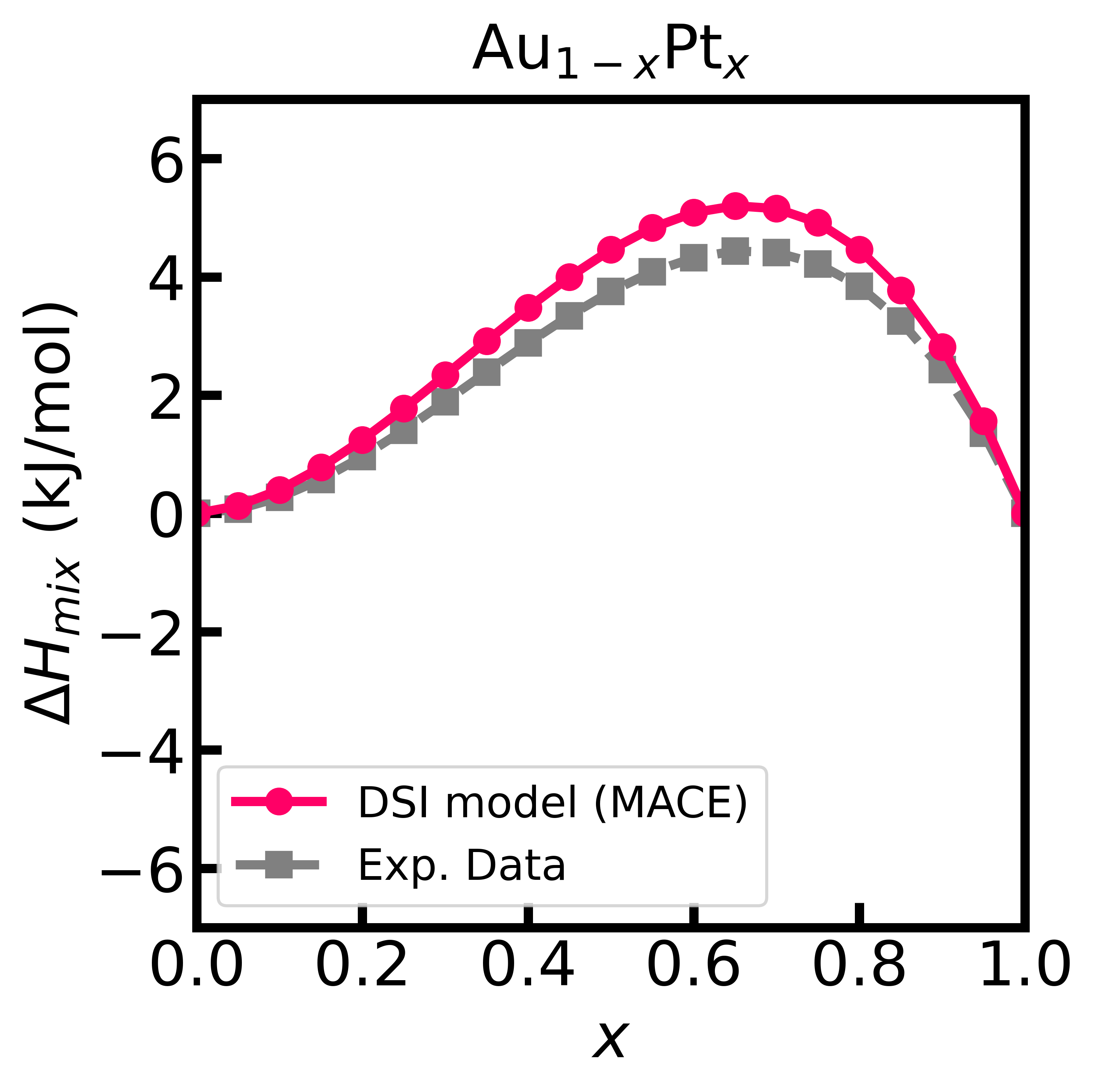
Figure 1 - Enthalpy of mixing of the Au-Pt alloy computed using the DSI model and MACE interatomic potentials.
DSI model from pre-calculated data
Using blendpy, we can also calculate the enthalpy of mixing for an alloy based on DFT simulations that are not initiated by the DSIModel class object. Instead, we can use external data for the total energies of the pristine and dilute supercell systems. For instance, using the ab initio simulation software GPAW,[^fn1] we calculate the total energies for the Au-Pt alloy using [3,3,3] supercells of Au and Pt (Atoms(Au27) and Atoms(Pt27)), as well as the dilute systems (Atoms(Au26Pt) and Atoms(Pt26Au)). These total energies are then used to construct the energy matrix (energy_matrix) in the following form:
energy_matrix = np.array([[ -85.940400,  -89.230299],   # [[  Au27, Au26Pt],
                          [-170.278459, -173.891172]])  #  [ Pt26Au,  Pt27]]
Next, we demonstrate how to calculate the enthalpy of mixing using the input energy matrix.
import numpy as np
import pandas as pd
import matplotlib.pyplot as plt
from ase.build import bulk
from ase.io import write
from blendpy import DSIModel

# Create the two bulk structures
gold = bulk('Au', 'fcc')
palladium = bulk('Pt', 'fcc')

# Write the structures to CIF files
write("cif_files/Au.cif", gold)
write("cif_files.Pt.cif", palladium)

# Create the DSI model
alloy_components = ['cif_files/Au.cif', 'cif_files/Pt.cif']
x0 = 1./27
blendpy= DSIModel(alloy_components=alloy_components, supercell=[3,3,3], x0=x0)

# Set the energy matrix
energy_matrix = np.array([[ -85.940400,  -89.230299],
                          [-170.278459, -173.891172]])

blendpy.set_energy_matrix(energy_matrix)

enthalpy= blendpy.get_enthalpy_of_mixing()

x = np.linspace(0, 1, len(enthalpy))

df_enthalpy = pd.DataFrame({'x': x, 'enthalpy': enthalpy})
In this case, it is MANDATORY to specify the minimum dilution factor (x0), the supercell size ([3,3,3]) used in the ab initio simulations, and the unit cell files ('Au.cif' and 'Pt.cif'). The unit cell files do not need to match exactly those used in the ab initio simulations.
Finally, we can plot the enthalpy of mixing and compare it with the experimental data.[^fn2]
# Plot the enthalpy of mixing
fig, ax = plt.subplots(1,1, figsize=(6,6))

ax.set_xlabel('x', fontsize=20)
ax.set_ylabel('$\Delta H_{mix}$ (kJ/mol)', fontsize=20)
ax.set_xlim(0,1)
ax.set_ylim(-7,7)
ax.set_xticks(np.linspace(0,1,6))
ax.set_yticks(np.arange(-6,7,2))
ax.set_title("Au$_{1-x}$Pt$_{x}$", fontsize=20, pad=10)

# plot data
# Experimental
df_exp = pd.read_csv("../../data/experimental/exp_AuPt.csv")
ax.plot(df_exp['x'], df_exp['enthalpy'], 's', color='grey', linestyle='--', linewidth=3, markersize=8, label="Exp. Data", zorder=1)

# DSI model
ax.plot(df_enthalpy['x'][::5], df_enthalpy['enthalpy'][::5], marker='o', color='#fc4e2a', markersize=8, linewidth=3, zorder=2, label="DSI model from DFT")

ax.legend(fontsize=16, loc='best')
ax.tick_params(axis='both', which='major', labelsize=20, width=3, length=8, direction='in')
ax.set_box_aspect(1)

for spine in ax.spines.values():
    spine.set_linewidth(3)

plt.tight_layout()
# plt.savefig('enthalpy_of_mixing_AuPt_from_input.png', dpi=400, bbox_inches='tight')
plt.show()
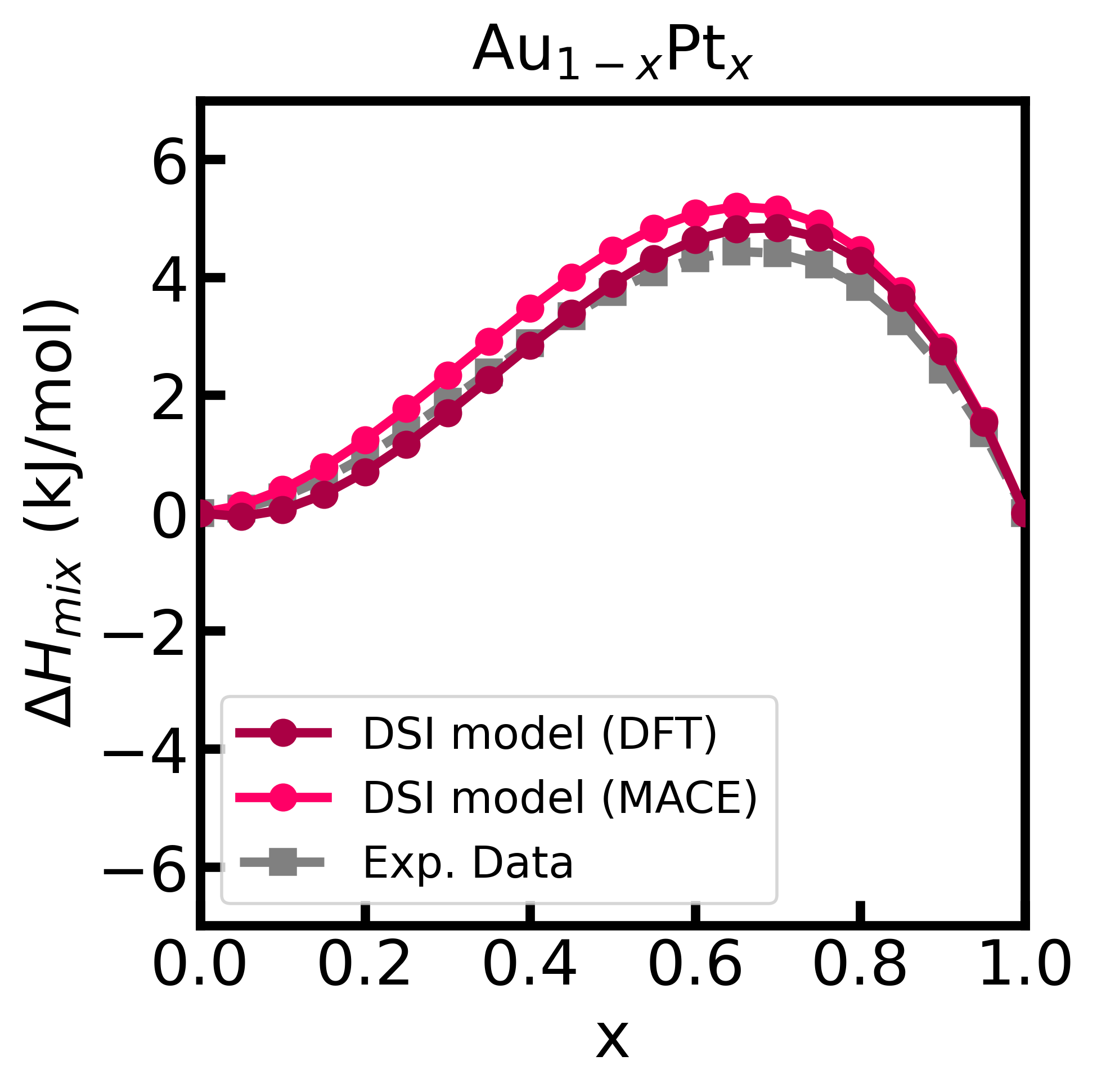
Figure 2 - Enthalpy of mixing of the Au-Pt alloy computed using the DSI model and energy matrix given from input (calculated with GPAW).
Polymorphism
Phase diagram (NOT WORKING)
By analyzing the mixing enthalpies and entropies, we can calculate the Gibbs free energy of the Au–Pt alloy mixture and determine both the spinodal and binodal (solvus) decomposition curves. These curves, which form key features of the alloy's phase diagram, delineate regions of differing stability: below the binodal curve, the solid solution (Au, Pt) is metastable, whereas it becomes unstable beneath the spinodal curve.
We begin by defining a temperature range over which to calculate the spinodal and binodal curves. Optionally, the results can be saved in CSV files.
temperatures = np.arange(300, 3001, 5)

# spinodal curve
df_spinodal = blendpy.get_spinodal_decomposition(temperatures = temperatures, npoints = 501)
df_spinodal.to_csv("data/phase_diagram/spinodal_AuPt.csv", index=False, header=True, sep=',')

# binodal curve
df_binodal = blendpy.get_binodal_curve(temperatures = temperatures, npoints=501)
df_binodal.to_csv("data/phase_diagram/binodal_AuPt.csv", index=False, header=True, sep=',')
To plot the phase diagram featuring the spinodal and binodal decomposition curves, we proceed as follows:
import pandas as pd

# Create figure and axis
fig, ax = plt.subplots(1,1, figsize=(8,8))

x = np.linspace(0, 1, 101)

# Configure axis labels and limits
ax.set_xlabel("$x$", fontsize=20)
ax.set_ylabel("$T$ (K)", fontsize=20)
ax.set_xlim(0,1)
ax.set_ylim(300, 2500)
ax.set_xticks(np.linspace(0,1,6))

# Plot the data
ax.plot(df_spinodal['x'], df_spinodal['t'], color='#d53e4f', linestyle='--', linewidth=3, label="Spinodal curve")
ax.plot(df_binodal['x'], df_binodal['t'], color='#d53e4f', linewidth=3, label="Binodal curve")

# Fill below the curves with transparency (alpha=0.3 means 30% opacity)
ax.fill_between(df_spinodal['x'], df_spinodal['t'], 300, color='#d53e4f', alpha=0.3)
ax.fill_between(df_binodal['x'], df_binodal['t'], 300, color='#d53e4f', alpha=0.3)
ax.legend(loc="best", fontsize=20)

# Add text annotations
ax.text(0.2, 1500, "Stable", fontsize=20, ha='center', va='center')
ax.text(0.4, 950, "Metastable", fontsize=20, ha='center', va='center', rotation=60)
ax.text(0.7, 700, "Unstable", fontsize=20, ha='center', va='center')

# Customize tick parameters
ax.tick_params(direction='in', axis='both', which='major', labelsize=20, width=3, length=8)
ax.set_box_aspect(1)
for spine in ax.spines.values():
    spine.set_linewidth(3)

plt.tight_layout()
# plt.savefig("phase_diagram.png", dpi=600, format='png', bbox_inches='tight')
plt.show()
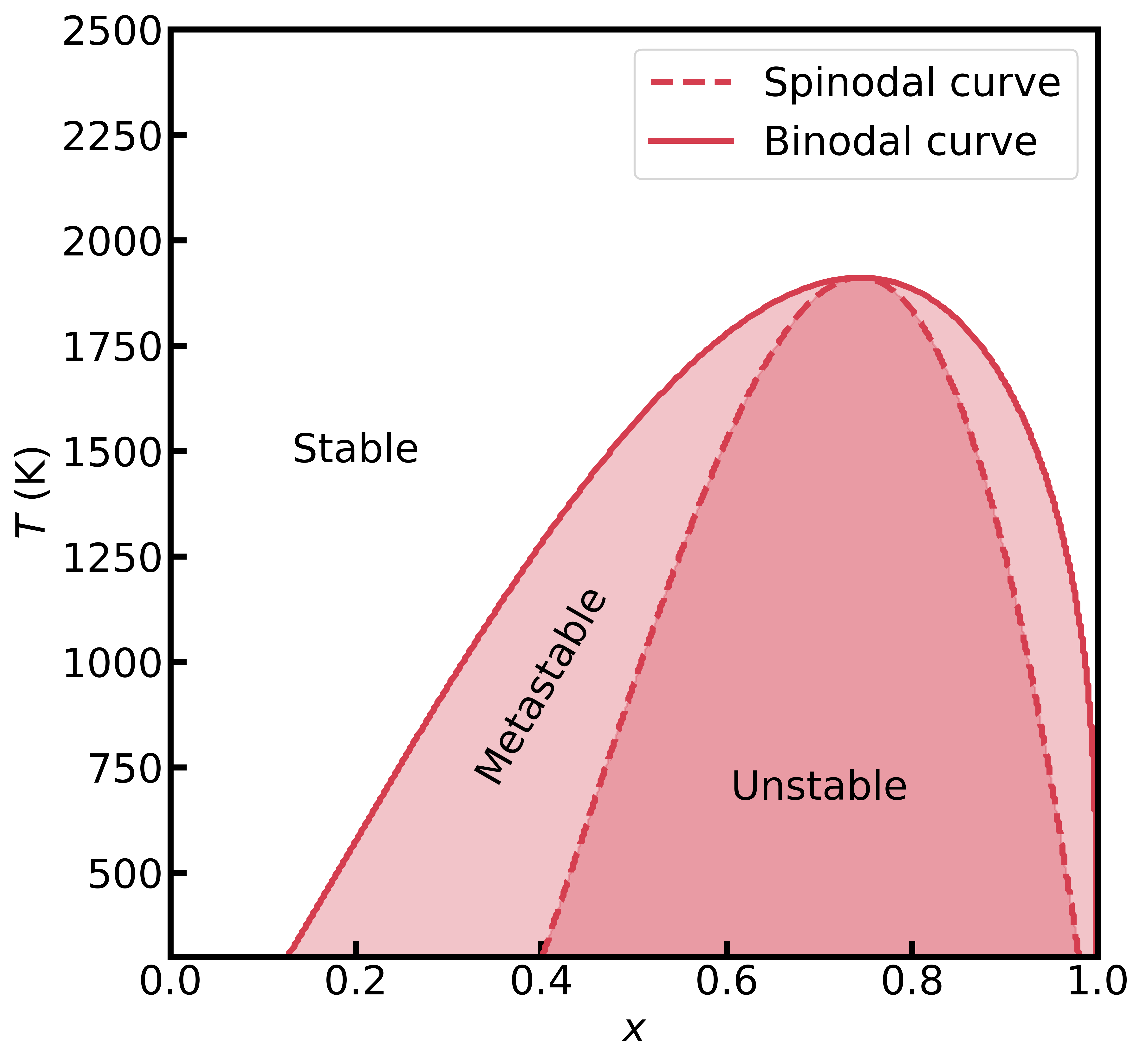
Figure 2 - Phase diagram of the Au–Pt alloy computed using the DSI model and MACE interatomic potentials.
License
This is an open source code under MIT License.
Acknowledgements
We thank financial support from FAPESP (Grant No. 2022/14549-3), INCT Materials Informatics (Grant No. 406447/2022-5), and CNPq (Grant No. 311324/2020-7).
References
[^fn1]: J. J. Mortensen et al., J. Chem. Phys. 160 092503 (2024).
[^fn2]: H. Okamoto and T. Massalski, Bull. Alloy Phase Diagr. 6, 229 (1985).
Release history Release notifications | RSS feed


Download files
Download the file for your platform. If you're not sure which to choose, learn more about installing packages.
Source Distribution
Built Distribution
Filter files by name, interpreter, ABI, and platform.
If you're not sure about the file name format, learn more about wheel file names.
Copy a direct link to the current filters
File details
Details for the file blendpy-25.3.42.tar.gz.
File metadata
- Download URL: blendpy-25.3.42.tar.gz
- Upload date:
- Size: 870.0 kB
- Tags: Source
- Uploaded using Trusted Publishing? No
- Uploaded via: twine/6.1.0 CPython/3.12.7
File hashes
| Algorithm | Hash digest | |
|---|---|---|
| SHA256 |
52d6671001733163a29154dd1bb9f13e7dc2126b11e85ae5370b514b0c814392
|
|
| MD5 |
b100ffd3c84f0d5c513b7d03cbc05e3e
|
|
| BLAKE2b-256 |
d6c1c486ab552ede598038be038a078d56d8b8ee664330757b4efc7ad99f72c5
|
File details
Details for the file blendpy-25.3.42-py3-none-any.whl.
File metadata
- Download URL: blendpy-25.3.42-py3-none-any.whl
- Upload date:
- Size: 31.6 kB
- Tags: Python 3
- Uploaded using Trusted Publishing? No
- Uploaded via: twine/6.1.0 CPython/3.12.7
File hashes
| Algorithm | Hash digest | |
|---|---|---|
| SHA256 |
4ef265288b756487af4a67419cb534b4099a6a83cc9bf92eefc2062bcde6da88
|
|
| MD5 |
7f7b173f7e7bc8bbc049aad47dc49495
|
|
| BLAKE2b-256 |
39b6dc26fa0d73a1f104f8cad1e7ea5307bc9126eef7052b6a8841cd1a4a5c99
|






