
ChemoMAE




ChemoMAE: A PyTorch toolkit for self-supervised spectral representation learning and spatial analysis of spectral differences.
Manuscript in preparation. A paper describing the method and its NIR-HSI case study of aged wood is being prepared. Links will be added when available.
- arXiv preprint: URL to be added.
- Research repository (GitHub): URL to be added.
This documentation describes ChemoMAE v0.2.3. See the release notes for changes to APIs, defaults, and saved artifacts from v0.2.2.
Why ChemoMAE?
When chemical states and their categories are not known in advance, spectral images can help explore where spectral differences occur and how they are organized in space. The representation used to compare spectra determines which differences become visible in that analysis.
ChemoMAE learns a low-dimensional representation from unlabeled spectra, then provides clustering and spatial evaluation tools for examining the resulting partitions. For hyperspectral images, retain the original pixel coordinates so that predicted labels can be placed back into each specimen's map. Spectral summaries and local chemical measurements can then support interpretation of the observed regions.
1. Learning through Masked Denoising
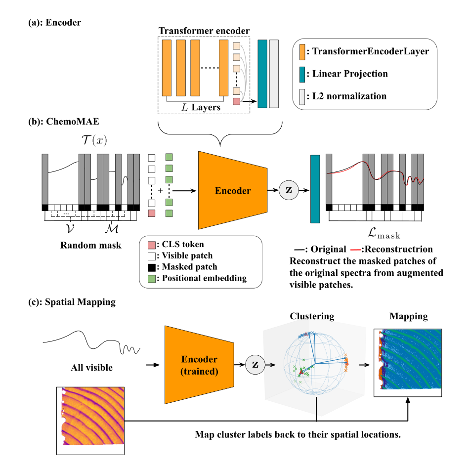
ChemoMAE divides a spectrum into contiguous patches and passes the visible patches, together with a CLS token, through a Transformer encoder. A decoder reconstructs all spectral channels from one latent vector. Trainer's default loss evaluates the hidden channels, encouraging the representation to capture relationships across spectral bands.
With SpectraAugmenter, the model receives a perturbed spectrum while the
reconstruction target remains the input before that additional perturbation.
This masked denoising task combines prediction of hidden bands with recovery
from specified spectral perturbations. The library also supports masked
reconstruction without augmentation and full-spectrum autoencoder training.
The manuscript uses a single affine decoder (decoder_num_layers=1). The
library supports both affine and MLP decoders; its default is a two-layer MLP
(decoder_num_layers=2). The examples below illustrate the library APIs.
2. Geometry for Comparing Spectral Shape
For nonconstant spectra with negligible eps, Standard Normal Variate (SNV)
centers each spectrum and scales it to approximately unit sample variance and a
common L2 norm. This emphasizes relative spectral shape. Constant spectra become
zero vectors, and finite eps makes the common-norm relation approximate.
Choose SNV when removing per-spectrum mean and scale is appropriate for the
measurement and analysis.
SpectraAugmenter provides fractional shift through channel interpolation
and tangent Gaussian noise through rotation in a random tangent direction.
Its default re-centering and norm restoration retain the geometry of
SNV-transformed inputs, so augmentation varies spectral shape without
reintroducing the removed mean and scale. These operations define controlled
perturbations; their relevance to actual measurement variation depends on the
chosen settings and application.
The encoder's projected latent vector is L2-normalized by default
(latent_normalize=True). Input spectra and latent vectors can therefore both
be compared by direction using cosine similarity. The latent vector has no
zero-mean constraint, and the learned mapping need not preserve input cosine
similarities. Set latent_normalize=False to retain unconstrained latents.
3. From Representations to Spatial Maps
After training, extract features with all patches visible and augmentation
disabled. CosineKMeans, used in the accompanying study, partitions feature
directions at a chosen observation granularity K. VMFMixture is an
additional option for probabilistic modeling of directional features. Cluster
IDs identify assignments; chemical meaning requires interpretation of the
spectra and supporting measurements.
For a spectral image, restore labels to their original pixel positions and use Local Label Agreement (LLA) to measure local spatial coherence beyond chance agreement implied by cluster occupancy. Cosine silhouette describes separation within the chosen representation. In the study, neither model training nor clustering uses spatial coordinates or neighbor relations, allowing the maps to be evaluated using spatial information held apart from fitting. For unseen-specimen evaluation, fit both the encoder and cluster centers on training specimens and keep them fixed during held-out prediction.
Quick Start
Install a CPU or CUDA build of PyTorch appropriate for your environment using the official installation selector, then install ChemoMAE v0.2.3:
python -m pip install "chemomae==0.2.3"
The package requires Python >=3.10 and PyTorch >=2.1. CI covers Python
3.10–3.13 with selected CPU PyTorch builds and a Python 3.10/PyTorch 2.1 lane;
it does not test every Python/PyTorch combination. If using PyTorch 2.1, keep
NumPy in the >=1.24,<2 range for its NumPy interoperability.
For an editable installation, clone the repository, check out v0.2.3, and run
the following from its root in your chosen environment:
python -m pip install -e .
ChemoMAE Example
The step-by-step workflow tutorial explains preprocessing, augmentation, epoch resume, clean evaluation, representations, streaming extraction, clustering, spatial maps, LLA, and saved artifacts. It uses small synthetic inputs. Settings illustrate API usage and are not a scientific benchmark protocol.
This compact CPU example defines all inputs and reloads the selected inference artifact before extracting features:
import tempfile
from pathlib import Path

import torch
from torch.utils.data import DataLoader, TensorDataset

from chemomae.preprocessing import snv
from chemomae.models import ChemoMAE
from chemomae.training import Trainer, TrainerConfig, Extractor, ExtractorConfig
from chemomae.clustering import CosineKMeans

torch.manual_seed(42)
data_stream = torch.Generator().manual_seed(7)
spectra = snv(torch.randn(80, 64, generator=data_stream))
train_x, test_x = spectra[:64], spectra[64:]

def loader(x: torch.Tensor) -> DataLoader:
    return DataLoader(TensorDataset(x), batch_size=16, shuffle=False)

device = torch.device("cpu")
run_dir = Path(tempfile.mkdtemp(prefix="chemomae-"))
model = ChemoMAE(
    seq_len=64, n_patches=8, n_mask=4, d_model=16,
    nhead=4, num_layers=1, latent_dim=8,
).to(device)
optimizer = torch.optim.AdamW(model.parameters(), lr=1e-3)
trainer = Trainer(
    model, optimizer, loader(train_x),
    cfg=TrainerConfig(
        out_dir=run_dir, device=device, resume_from=None, use_ema=False,
        progress=False, verbose=False,
    ),
)
trainer.fit(epochs=2)

inference_model = ChemoMAE.load(run_dir / "last_model.artifact.pt", device=device)
extractor = Extractor(
    inference_model,
    ExtractorConfig(representation="normalized_latent", output_device="cpu"),
)
train_features = extractor(loader(train_x))
test_features = extractor(loader(test_x))

clusterer = CosineKMeans(n_components=3, max_iter=30, device=device, random_state=42)
clusterer.fit(train_features)
test_labels = clusterer.predict(test_features)
clusterer.save_centroids(run_dir / "clusters.pt")
print(test_labels, clusterer.converged_, clusterer.stop_reason_)
For custom masks, batch ordering, schedules, and caller-owned RNG state, use the public Trainer hooks or plain PyTorch loop. Model persistence explains inference artifacts and training checkpoints. API documentation covers the full library.
Library Features
chemomae.preprocessing
SNVScaler
SNVScaler performs row-wise mean subtraction and variance scaling. Each
spectrum is divided by its sample standard deviation (ddof=1 for L>=2)
plus eps; length-one spectra use ddof=0.
It is a stateless transformer supporting NumPy and PyTorch. Torch
normalization and statistics stay on the input device and retain autograd;
float64 is preserved and float16/bfloat16 inputs are promoted to float32.
When transform_stats=True, it returns (Y, mu, sd), where sd already includes eps and can be directly used for inverse reconstruction.
Nonconstant rows have approximately unit sample variance when eps is negligible,
and an L2 norm near sqrt(L - 1). Constant and length-one spectra produce zeros;
they do not define a direction on that hypersphere.
import numpy as np
from chemomae.preprocessing import SNVScaler

X = np.array([[1.0, 2.0, 3.0],
              [4.0, 5.0, 6.0]], dtype=np.float32)

scaler = SNVScaler()
Y = scaler.transform(X)

scaler = SNVScaler(transform_stats=True)
Y, mu, sd = scaler.transform(X)
X_rec = scaler.inverse_transform(Y, mu=mu, sd=sd)
Key Features
- unbiased standard deviation (
ddof=1, with automatic fallback forL=1) - numerically stable
epshandling - native on-device Torch arithmetic and same-framework statistics
- explicit precision: float32/float64 preserved, half precision promoted to float32
When to Use
- comparing relative spectral shapes when per-spectrum mean and scale should be removed
- preparing spectra for directional analysis under that preprocessing choice
cosine_fps_downsample
cosine_fps_downsample performs Farthest-Point Sampling (FPS) using cosine
dissimilarity. Starting from one sampled row, it greedily adds the row with the
greatest cosine distance to its nearest selected row. It is an optional way to
cover spectral directions with fewer rows; the selected subset does not preserve their density
or spatial distribution.
Internally, all rows are L2-normalized for selection, but the returned subset is drawn from the original-scale input X.
It supports NumPy and PyTorch inputs with an explicit computation device.
The default follows a Torch input's device, or uses CPU for NumPy input.
import numpy as np
from chemomae.preprocessing import cosine_fps_downsample

X = np.random.randn(1000, 128).astype(np.float32)
X_sub = cosine_fps_downsample(X, ratio=0.1, seed=42)
Pass device="cuda" to request GPU computation, or device="cpu" to keep it
on CPU. A caller-owned generator may replace seed for initial-point control.
Key Features
- internal normalization for cosine-based selection
- output kept in original scale
- device-aware Torch support
When to Use
- diversity-driven subsampling
- reducing redundancy in large spectral datasets
chemomae.models
ChemoMAE
ChemoMAE is a Masked Autoencoder for 1D spectra.
Contiguous spectral bands are grouped into patches and masked at the patch level.
The encoder processes the visible patch tokens together with a CLS token.
The CLS output is projected to a latent_dim vector, and the decoder
reconstructs the full spectrum from that single bottleneck. Use
decoder_num_layers=1 for the manuscript's affine decoder or a larger value for
an MLP; the library default is 2.
Optional L2 normalization expresses the latent representation as a direction for cosine comparison. Train with hidden-band loss to learn cross-band relationships, then extract all-visible features for downstream analysis.
import torch
from chemomae.models import ChemoMAE

mae = ChemoMAE(
    seq_len=256,
    d_model=256,
    nhead=4,
    num_layers=4,
    dim_feedforward=1024,
    decoder_num_layers=2,
    latent_dim=8,
    latent_normalize=True,
    n_patches=32,
    n_mask=16,
)

x = torch.randn(8, 256)
x_rec, z, visible = mae(x)
Key Features
- patch-wise masking
- Transformer encoder over visible tokens
- configurable affine or MLP decoder
- optional L2-normalized latent
- cosine-friendly embeddings
When to Use
- learning spectral representations through masked reconstruction or masked denoising
- downstream clustering, visualization, or supervised fine-tuning
chemomae.training
build_optimizer & build_scheduler
Utility functions for configurable AdamW optimization and learning-rate scheduling.
build_optimizercreates grouped AdamWbuild_schedulercreates linear warmup → cosine decay
from chemomae.models import ChemoMAE
from chemomae.training import build_optimizer, build_scheduler

import torch

device = torch.device("cpu")
model = ChemoMAE(seq_len=256).to(device)
optimizer = build_optimizer(model, lr=1.0e-3, weight_decay=0.05)
scheduler = build_scheduler(
    optimizer,
    steps_per_epoch=len(train_loader),
    epochs=100,
    warmup_epochs=5,
)
Inspect optimizer.param_groups for actual decay exclusions. The scheduler
sets a positive initial warmup rate at construction and advances after successful
updates; its post-step LR belongs to the next update. See the
optimizer/scheduler guide for the exact indexing.
When to Use
- building AdamW parameter groups with explicit weight-decay exclusions
- scheduling warmup and cosine decay over successful optimizer updates
SpectraAugmenterConfig & SpectraAugmenter
SpectraAugmenter provides SNV-geometry-aware augmentation for SNV-normalized spectra.
SNV-transformed nonconstant spectra are mean-centered with approximately a common norm. The default augmentation settings retain that geometry by:
- re-centering each spectrum to mean zero
- re-normalizing each spectrum to the original per-spectrum L2 norm
The current implementation supports two augmentations:
-
fractional shift A small wavelength-axis perturbation implemented by interpolation.
-
tangent Gaussian noise A random local perturbation constructed by projecting Gaussian noise onto the tangent space and rotating the spectrum by a sampled angle.
Fractional shift is controlled by shift_delta_range, while tangent Gaussian noise is controlled by noise_angle_deg_range.
For masked denoising, augmentation is applied before patch masking, while the target remains the spectrum before augmentation. Keeping mean and norm fixed allows these operations to vary spectral shape without restoring the offsets and scale that SNV removed. Choose strengths for the intended application; mean and norm preservation alone does not ensure chemical-state preservation.
from chemomae.training import SpectraAugmenter, SpectraAugmenterConfig

aug_cfg = SpectraAugmenterConfig(
    shift_prob=0.5,
    shift_delta_range=(-2.0, 2.0),
    noise_prob=0.5,
    noise_angle_deg_range=(0.5, 3.0),
    shuffle_order_per_batch=True,
    recenter_after_each_op=True,
    renorm_to_input_norm=True,
    eps=1.0e-8,
)

augmenter = SpectraAugmenter(aug_cfg)

augmenter.train()
x_aug = augmenter(x)
Key Features
- SNV-compatible spectral augmentation
- fractional wavelength-axis shift
- tangent-space Gaussian perturbation
- probability-controlled operation application
- delta-controlled fractional shift
- angle-controlled tangent Gaussian noise
- optional random ordering of shift/noise operations
- optional re-centering to zero mean after each operation
- optional re-normalization to the input L2 norm after each operation
- implemented as
nn.Module, so it supports.to(device) - automatically inactive in
eval()mode
Mode Behavior
SpectraAugmenter applies augmentation only in train() mode.
augmenter.train()
x_aug = augmenter(x)  # augmentation is applied

augmenter.eval()
x_same = augmenter(x)  # input is returned unchanged
This behavior is important when using the augmenter outside the Trainer.
For example, Extractor and Tester temporarily set the augmenter to train() when augmentation is explicitly requested, while keeping the ChemoMAE model itself in eval() mode.
When to Use
- during ChemoMAE pretraining on SNV-normalized spectra
- when you want denoising-style pretraining, where the model receives weakly perturbed spectra but reconstructs the original spectra
- when evaluating reconstruction robustness under controlled spectral perturbations
- when extracting augmented latent representations for robustness checks or test-time augmentation style analysis
- when perturbations should remain compatible with cosine-based or hyperspherical downstream analysis
TrainerConfig & Trainer
TrainerConfig and Trainer form the core training engine of ChemoMAE.
They provide a fixed-budget training loop with an explicit choice between masked-only and full-spectrum reconstruction loss, with support for:
- AMP (
bf16/fp16) - optional TF32
- EMA parameter tracking
- optional
SpectraAugmenter loss_region="masked"(default) orloss_region="all"- gradient clipping
- checkpointing and resume
- weights-only export for final model variants
- JSON history logging
When an augmenter is supplied, the default preparation step perturbs the model input and retains the original batch as the reconstruction target. This supports the masked denoising task without requiring labels or spatial coordinates.
ChemoMAE does not use validation-loss-based early stopping or best-checkpoint selection.
fit(epochs=...) uses an absolute epoch budget. Configure the scheduler against
successful optimizer updates; the Trainer does not provide a direct step budget.
Select and reload the final raw or EMA export before downstream inference.
The following feature snippet assumes the caller supplies train_loader with
spectra of length 256. The complete synthetic workflow appears above and in the
linked tutorial.
from chemomae.models import ChemoMAE
from chemomae.training import (
    Trainer,
    TrainerConfig,
    SpectraAugmenter,
    SpectraAugmenterConfig,
    build_optimizer,
    build_scheduler,
)

import torch

device = torch.device("cpu")
model = ChemoMAE(seq_len=256, latent_dim=16, n_patches=32, n_mask=24).to(device)

cfg = TrainerConfig(
    out_dir="runs",
    device=str(device),
    amp=False,
    amp_dtype="bf16",
    enable_tf32=False,
    grad_clip=1.0,
    use_ema=True,
    ema_decay=0.999,
    loss_type="mse",
    loss_region="masked",
    reduction="mean",
    resume_from=None,
)

aug_cfg = SpectraAugmenterConfig(
    shift_prob=0.5,
    shift_delta_range=(-2.0, 2.0),
    noise_prob=0.5,
    noise_angle_deg_range=(0.5, 3.0),
    shuffle_order_per_batch=True,
    recenter_after_each_op=True,
    renorm_to_input_norm=True,
)
augmenter = SpectraAugmenter(aug_cfg)

optimizer = build_optimizer(model, lr=1.0e-3, weight_decay=0.05)

epochs = 800
scheduler = build_scheduler(
    optimizer,
    steps_per_epoch=len(train_loader),
    epochs=epochs,
    warmup_epochs=40,
)

trainer = Trainer(
    model,
    optimizer,
    train_loader,
    scheduler=scheduler,
    augmenter=augmenter,
    cfg=cfg,
)

result = trainer.fit(epochs=epochs)
model.load_state_dict(torch.load(
    "runs/" + result["final_model"], map_location=device, weights_only=True,
))
model.eval()
For full-spectrum autoencoder training, use n_mask=0 together with loss_region="all". The loss region is never inferred from n_mask.
Key Features
- model-device defaults with AMP disabled; explicit CUDA/precision opt-in
- explicit epoch-budget SSL pretraining
- EMA tracking after each successful optimizer update
- EMA-consistent final export behavior:
- final raw weights →
last_model.pt - final EMA weights →
ema_last_model.ptif EMA is enabled - config-and-weights bundles →
last_model.artifact.ptandema_last_model.artifact.pt
- final raw weights →
checkpoints/last.ptstores versioned training state and standard global RNG- independently configurable history/checkpoint/export paths and progress/summary controls
- optional train-time spectral augmentation
- scheduler stepping after successful optimizer updates
- public preparation/event/checkpoint hooks and separate update/skip counters
- atomic JSON history logging
Outputs
runs/
├── training_history.json
│    ↳ Per-epoch records:
│       [
│         {
│           "epoch": 1,
│           "train_loss": ...,
│           "lr": ...,
│           "time_sec": ...,
│           "loss_region": "masked",
│           "n_mask": 24
│         },
│         ...
│       ]
│
├── last_model.pt
│    ↳ Final raw model weights at the end of training
├── last_model.artifact.pt
│    ↳ Full constructor configuration and selected raw weights
│
├── ema_last_model.pt
│    ↳ Final EMA weights at the end of training
│       (saved only when EMA is enabled)
├── ema_last_model.artifact.pt
│    ↳ Full constructor configuration and selected EMA weights
│
└── checkpoints/
     └── last.pt
          ↳ Full checkpoint for resume:
             config + model + optimizer + scheduler + scaler + EMA
             + loss policy + history + progress + global RNG + extension state
These are the default paths. Each output can be relocated or disabled through
TrainerConfig; setting model_artifacts=False disables the inference bundles.
See the artifact guide for loading and resume rules.
When to Use
- fixed-budget masked reconstruction pretraining for ChemoMAE
- full-spectrum autoencoder training with
n_mask=0andloss_region="all" - validation-free SSL pretraining
- training runs where model selection is handled by an explicit final rule, such as EMA-last weights
TesterConfig & Tester
Tester provides a lightweight evaluation loop for trained ChemoMAE models.
It computes masked or full-spectrum reconstruction loss over a DataLoader, with explicit AMP, optional fixed visible masks/augmentation, and JSON logging. Reductions aggregate errors across the complete loader rather than re-averaging batch losses; empty selected regions and empty loaders raise errors. Reconstruction error describes the prediction task. Evaluate the spatial maps and their chemical interpretation separately from this loss.
from chemomae.training import Tester, TesterConfig

cfg = TesterConfig(
    out_dir="runs",
    device="cuda",
    amp=True,
    amp_dtype="bf16",
    loss_type="mse",
    reduction="mean",
    fixed_visible=None,
    log_history=True,
    history_filename="test_history.json",
)

tester = Tester(
    model,
    cfg,
    augmenter=None,
)

avg_loss = tester(test_loader)
print("Test loss:", avg_loss)
When augmenter is provided, Tester evaluates reconstruction from augmented inputs while keeping the reconstruction target as the original spectrum.
tester = Tester(
    model,
    cfg,
    augmenter=augmenter,
)
When to Use
- evaluating masked reconstruction loss
- comparing reconstruction behavior under fixed visible masks
- evaluating robustness to weak spectral perturbations
- logging test losses separately from training history
ExtractorConfig & Extractor
Extractor provides a latent extraction pipeline from trained ChemoMAE models in all-visible mode.
It directly calls the encoder with an all-visible mask, so ChemoMAE masking is not used during extraction. Without an augmenter, this gives deterministic latent embeddings with respect to masking.
Use the selected inference artifact to extract features before fitting a clusterer. Retain the association between rows, specimens, and pixel coordinates when those features will be used to construct spatial maps.
It supports AMP inference, Torch/NumPy return types, optional saving, and optional SpectraAugmenter.
from chemomae.training import Extractor, ExtractorConfig

cfg = ExtractorConfig(
    device="cuda",
    amp=True,
    amp_dtype="bf16",
    save_path=None,
    representation="normalized_latent",
    output_type="numpy",
    output_device="cpu",
)

extractor = Extractor(
    model,
    cfg,
    augmenter=None,
)

Z = extractor(loader)
For large outputs, stream batches instead of retaining the whole feature array:
for features in extractor.iter_transform(loader):
    # Consume features here or write them to your own storage.
    print(features.shape)
output_type="tensor" and output_device="cuda" retain batches on GPU.
Choose representation="cls", "raw_latent", "normalized_latent", or
"latent" (configured model normalization). Direct model.encode(x, ...)
offers the same representations without decoder execution or random masking.
When augmenter is provided, Extractor applies augmentation before encoder inference.
extractor = Extractor(
    model,
    cfg,
    augmenter=augmenter,
)

Z_aug = extractor(loader)
With an augmenter, extracted embeddings may vary across calls because spectral shift/noise augmentation can be stochastic.
When to Use
- extracting latents for clustering
- visualization
- downstream analysis
- robustness checks using augmented latent embeddings
chemomae.clustering
CosineKMeans & elbow_ckmeans
CosineKMeans implements hyperspherical k-means with cosine similarity and
unit-norm nonzero centroids. It quantizes spectral feature directions into K
assignments. K controls the granularity of the resulting map, and the cluster
IDs carry no predefined chemical meaning. elbow_ckmeans provides an exploratory
candidate from the inertia curve.
import torch
from chemomae.clustering import CosineKMeans, elbow_ckmeans

X = torch.randn(10_000, 64)
ckm = CosineKMeans(n_components=12, device="cuda", random_state=42)
ckm.fit(X)
labels = ckm.predict(X)
When to Use
- clustering unit-sphere embeddings
- examining partitions at prescribed values of
Kor exploring an inertia curve
VMFMixture & elbow_vmf
VMFMixture fits a von Mises–Fisher mixture model on the unit hypersphere,
estimating component directions, concentrations, weights, and soft
responsibilities. It is an additional library option; the accompanying study
uses CosineKMeans for its main analysis.
The implementation uses CPU float64 scaled Bessel calculations with an
underflow-safe series fallback and retains valid unit directions for degenerate
components. lower_bound_ describes the final model; converged_ and
stop_reason_ distinguish tolerance, likelihood decrease, and iteration limit.
The concentration update remains approximate. The linked documentation explains
precision, persistence, and the interpretation of elbow_vmf.
import torch
from chemomae.clustering import VMFMixture, elbow_vmf

X = torch.randn(10000, 64, device="cuda")
vmf = VMFMixture(n_components=16, device="cuda", random_state=42)
vmf.fit(X)
labels = vmf.predict(X)
When to Use
- probabilistic clustering of unit-sphere embeddings
- comparing directional mixture fits using BIC or NLL curves
silhouette_samples_cosine_gpu & silhouette_score_cosine_gpu
Cosine silhouette metrics on CPU or CUDA describe within-cluster compactness relative to separation from other clusters in the supplied representation. Use them as a diagnostic alongside spatial maps and occupancy; separation in feature space and spatial coherence describe different properties.
import numpy as np
from chemomae.clustering import silhouette_score_cosine_gpu

X = np.random.randn(100, 16).astype(np.float32)
labels = np.random.randint(0, 4, size=100)

score = silhouette_score_cosine_gpu(X, labels, device="cpu")
print(score)
When to Use
- inspecting separation within a spectral or latent representation
- comparing partitions at different observation granularities
local_label_agreement
local_label_agreement measures local spatial coherence beyond the chance
agreement implied by cluster occupancy. Its corrected .score follows the
definition in the linked document; .raw_agreement is reported separately.
Binary class-map convolution supports CPU/CUDA and class chunking. Explicit
masks exclude background without reserving label zero, and only valid neighbor
pairs within the image contribute. Results include directed-pair integer counts,
occupancy, and reasons for undefined scores.
from chemomae.clustering import local_label_agreement

label_map = np.array([[0, 0, 0, 8]], dtype=np.int64)
valid_mask = np.ones_like(label_map, dtype=bool)
result = local_label_agreement(label_map, valid_mask, device="cpu")
for window in result.windows:
    print(window.window, window.score, window.undefined_reasons)
When to Use
- evaluating predicted label maps at specified neighborhood widths
- assessing coherence using an image's original pixel relationships
chemomae.utils
set_global_seed
Unified seeding for Python, NumPy, and PyTorch, with optional CuDNN determinism.
from chemomae.utils import set_global_seed

set_global_seed(42)
When to Use
- at the start of any experiment
- before training, testing, clustering, or extraction
License
ChemoMAE is released under the Apache License 2.0, a permissive open-source license that allows both academic and commercial use with minimal restrictions.
You are free to:
- use the code
- modify it
- distribute modified or unmodified versions
provided that the original copyright notice and license text are preserved.
The software is provided “as is”, without warranty of any kind.
For complete terms, see the official license text: https://www.apache.org/licenses/LICENSE-2.0
1 maintainer

Metadata
1 maintainer
Release files for chemomae 0.2.3
For a detailed explanation of source distributions (sdists) and built distributions (wheels), please see the package formats documentation.
Source distribution (sdist)
| File | Size | Uploaded | |
|---|---|---|---|
| chemomae-0.2.3.tar.gz | 108.9 kB | Details |
Built distribution (wheel)
| File | Interpreter | ABI | Platform | Reset |
|---|---|---|---|---|
| chemomae-0.2.3-py3-none-any.whl | Python 3 | none | any | Details |
Total release size: 207.5 kB
Release files / chemomae-0.2.3.tar.gz
| Download URL | chemomae-0.2.3.tar.gz |
|---|---|
| Size | 108.9 kB |
| Tags | Source |
|
SHA-256 checksum How to use checksums |
babc90205ae4e220b53db4d3da1ee5fd5b2339a710dbeaafb8e9fd2248d4ef0d
|
|
BLAKE2b-256 checksum How to use checksums |
36f5ff90b7d0dc1a2d04e3065a13e350704658df3dea11e82d6c2f3118dab23b
|
| Upload date | |
|
Uploaded using Trusted Publishing? What is trusted publishing? |
No |
| Uploaded via |
twine/7.0.0 CPython/3.13.14
|
Release files / chemomae-0.2.3-py3-none-any.whl
| Download URL | chemomae-0.2.3-py3-none-any.whl |
|---|---|
| Size | 98.6 kB |
| Tags | Python 3 |
|
SHA-256 checksum How to use checksums |
0d27d5c450309fbd073b6cdbfd4c5d0ee2fbd5dd1618336b7e5f66cc2c1fa4ce
|
|
BLAKE2b-256 checksum How to use checksums |
4b81a737362046f208012027094cbbf386e1136a71ed06883e64a74f746e8935
|
| Upload date | |
|
Uploaded using Trusted Publishing? What is trusted publishing? |
No |
| Uploaded via |
twine/7.0.0 CPython/3.13.14
|














