
Chromatic Confocal Sensor Ray Tracer
Specialized ray tracing engine designed for simulating and optimizing chromatic confocal sensors. This repository provides a powerful toolset for researchers and engineers working on precise optical measurement systems, enabling the accurate modeling of light interactions within chromatic confocal setups.
Installation
The library can be simply installed by:
pip install confocal-raytracer
Defining the setup
The optical setup is defined inside a JSON-like file. If, for example, an achromatic doublet is defined each face of both lenses should be defined as follows:
doublet = {
    "AC500-150-A-ML_1": {
        "Front Face": dict(
            curvature=96.85, konic=0, z_0=0, aperture_radius=50 / 2
        ),
        "Back Face": dict(
            curvature=-73.74,
            konic=0,
            z_0=9.5,
            aperture_radius=50 / 2,
        ),
        "Material": "BAK4",
        "Calibration": False,
    },
    "AC500-150-A-ML_2": {
        "Front Face": dict(
            curvature=-73.74, konic=0, z_0=9.5, aperture_radius=50 / 2
        ),
        "Back Face": dict(
            curvature=-241.63,
            konic=0,
            z_0=13.5,
            aperture_radius=50 / 2,
        ),
        "Material": "SF10",
        "Calibration": False,
    },
    "AC500-150-A-ML_1_R": {
        "Front Face": dict(
            curvature=241.63,
            konic=0,
            z_0=0,
            aperture_radius=50 / 2,
        ),
        "Back Face": dict(
            curvature=73.74, konic=0, z_0=4, aperture_radius=50 / 2
        ),
        "Material": "BAK4",
        "Calibration": False,
    },
    "AC500-150-A-ML_2_R": {
        "Front Face": dict(
            curvature=73.74,
            konic=0,
            z_0=4,
            aperture_radius=50 / 2,
        ),
        "Back Face": dict(
            curvature=-96.85, konic=0, z_0=13.5, aperture_radius=50 / 2
        ),
        "Material": "SF10",
        "Calibration": False,
    },
    "Sensor": {
        "Front Face": dict(
            curvature=float("inf"),
            konic=0,
            z_0=170,
            aperture_radius=100,
        ),
        "Back Face": dict(
            curvature=float("inf"),
            konic=0,
            z_0=170,
            aperture_radius=100,
        ),
        "Material": "SF2",
        "Calibration": False,
    },
}
Lens materials
The materials available with their refractive indexes should be specified in a Pandas Data Frame. The custom spectrum intensity can also be specified in the same Data Frame as follows:
| wl_nm | intensity | n_BK7 | n_SF2 | n_SF5 | n_BAF10 | n_SF10 | n_BAK4 | n_SF57 |
|---|---|---|---|---|---|---|---|---|
| 500.5 | 0.0851431638 | 1.5213856439764 | 1.6587264318676913 | 1.6847781738090497 | 1.67825 | 1.74315 | 1.57468 | 1.86746 |
| 500.7 | 0.08645302802 | 1.5213723632237195 | 1.6586929033319964 | 1.6847437966326086 | 1.6782202524647911 | 1.7430968741556505 | 1.574659846238762 | 1.8673847333525386 |
| 500.8 | 0.08502408117 | 1.5213657288620468 | 1.658676166909398 | 1.684726608044388 | 1.6782055071330022 | 1.7430704823647605 | 1.5746498284981434 | 1.8673473595993073 |
| 501.0 | 0.08721513301 | 1.5213524721680336 | 1.6586427497546976 | 1.6846922308679468 | 1.6781762683497092 | 1.7430180354906653 | 1.5746299095672376 | 1.86727312240276 |
| 501.1 | 0.08640539646 | 1.5213458498356942 | 1.658626069022597 | 1.684675042279726 | 1.6781617729016662 | 1.7429919781855066 | 1.5746200076850838 | 1.867236255427011 |
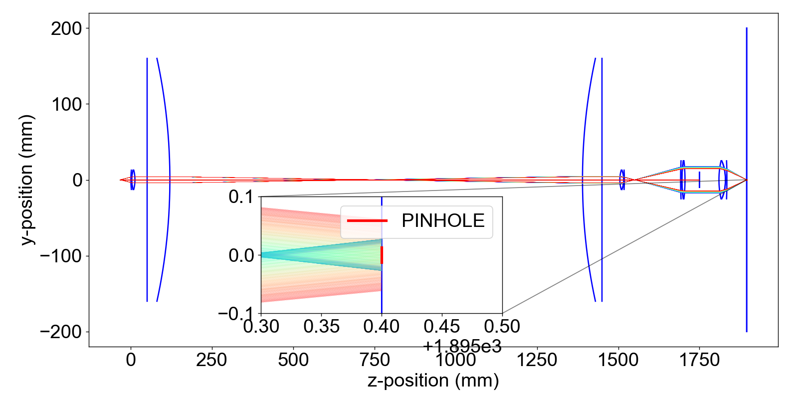
Example usage
from confocal_raytracer.simulation.raytrace import RayTrace
from confocal_raytracer.simulation.setup import chromatic_confocal
from confocal_raytracer.simulation._utils import plotter
from confocal_raytracer.load_data import n_data
import numpy as np
import matplotlib.pyplot as plt
import time
import warnings


# Ignore warning in axins legend location.
warnings.filterwarnings("ignore")

# Set refractive index of the spatial filter
n_data["n_absorb"] = np.inf

# Decimate the refractive index data to make
# the plot faster
n_data = n_data[::5]

# Get example optical data
optical_data = chromatic_confocal

# Set the pinhole size before sensor
PINHOLE_SIZE = 25 / 1000  # milimeters

# Number of rays from light source
N_RAYS = 3
# Set the extension of the light source
LIGHT_SOURCE_RADIUS = 0 / 1000  # milimeters
# Set the desviation angle with respecto to the
# optical axis of the N_RAYS
THETA = 6.0  # Degrees
# If LIGHT_SOURCE_RADIUS != 0 it is possible to set
# more rays for each height with the same desviation angle
N_RAYS_HEIGHT = 1
# Light source position
Z0 = -33.4  # Light source position same as
# back focal length of the achormatic doublet

fig, ax = plt.subplots()

# RayTrace object
raytrace = RayTrace(
    optical_data=optical_data,
    n_data=n_data,
    light_source_radius=LIGHT_SOURCE_RADIUS,
    n_rays=N_RAYS,
    theta=THETA,
    z0=Z0,
    n_rays_height=N_RAYS_HEIGHT,
)

t0 = time.perf_counter()
# After intersecting the full system,
# frays will have the shape (len(n_data), N_RAYS_HEIGHT, N_RAYS)
# where each one of the rays will be a Ray object with all the
# parameters included in it such as: angle of incidence and path followed by the ray
frays = raytrace.intersect_full_system()
print("Elapsed time (s): ", time.perf_counter() - t0)

# Plot setup
fig, ax = plotter(optical_data=optical_data, final_rays=frays, fig=fig, ax=ax)
plt.plot(
    [
        optical_data["Sensor"]["Front Face"]["z_0"],
        optical_data["Sensor"]["Front Face"]["z_0"],
    ],
    [-PINHOLE_SIZE / 2, PINHOLE_SIZE / 2],
    c="r",
)
ax.set(xlabel="z-position (mm)", ylabel="y-position (mm)")
axins = ax.inset_axes([0.25, 0.1, 0.35, 0.35])
plotter(optical_data=optical_data, final_rays=frays, fig=fig, ax=axins)
axins.plot(
    [
        optical_data["Sensor"]["Front Face"]["z_0"],
        optical_data["Sensor"]["Front Face"]["z_0"],
    ],
    [-PINHOLE_SIZE / 2, PINHOLE_SIZE / 2],
    c="r",
    lw=3,
    label="PINHOLE",
)
x1, x2, y1, y2 = (
    optical_data["Sensor"]["Front Face"]["z_0"] - 0.1,
    optical_data["Sensor"]["Front Face"]["z_0"] + 0.1,
    -0.1,
    0.1,
)
axins.legend()
axins.set_xlim(x1, x2)
axins.set_ylim(y1, y2)
plt.gca().indicate_inset_zoom(axins, edgecolor="black")
plt.tight_layout()
plt.show()
1 maintainer

Metadata
1 maintainer
Release files for confocal-raytracer 0.1.34
For a detailed explanation of source distributions (sdists) and built distributions (wheels), please see the package formats documentation.
Source distribution (sdist)
| File | Size | Uploaded | Provenance | Actions |
|---|---|---|---|---|
| confocal_raytracer-0.1.34.tar.gz | 300.9 kB | Without provenance | Details for confocal_raytracer-0.1.34.tar.gz |
Built distribution (wheel)
| File | Interpreter | ABI | Platform | Actions Reset |
|---|---|---|---|---|
| confocal_raytracer-0.1.34-py3-none-any.whl | Python 3 | none | any | Details for confocal_raytracer-0.1.34-py3-none-any.whl |
Total release size: 594.2 kB
Release files / confocal_raytracer-0.1.34.tar.gz
| Download URL | confocal_raytracer-0.1.34.tar.gz |
|---|---|
| Size | 300.9 kB |
| Tags | Source |
|
SHA-256 checksum How to use checksums |
01e33583f2417b3d5ca2592ab9e451520a6110dd354ae15315a5aaf090ecceba
|
|
BLAKE2b-256 checksum How to use checksums |
13f154a6e17ccfbef39f607c490213c6f080b86f6be30777b444ff13e1d9b885
|
| Upload date | |
|
Uploaded using Trusted Publishing? What is trusted publishing? |
No |
| Uploaded via |
poetry/1.8.2 CPython/3.9.13 Windows/10
|
Release files / confocal_raytracer-0.1.34-py3-none-any.whl
| Download URL | confocal_raytracer-0.1.34-py3-none-any.whl |
|---|---|
| Size | 293.2 kB |
| Tags | Python 3 |
|
SHA-256 checksum How to use checksums |
92edc9689b94cde9e595a4cd9dd33cb12b2ceedc54fb1a555a0001137e536232
|
|
BLAKE2b-256 checksum How to use checksums |
bb868c1ef126ce73746e3f48025b4812a1df8ee1137bee4b1edea63394aec366
|
| Upload date | |
|
Uploaded using Trusted Publishing? What is trusted publishing? |
No |
| Uploaded via |
poetry/1.8.2 CPython/3.9.13 Windows/10
|
Security for confocal-raytracer 0.1.34
Provenance
Provenance describes where a file came from. On PyPI, provenance is shared via attestations, which provide a verifiable record of the build or publishing details. View details, limitations and caveats.
No provenance found
None of the files in this release were uploaded with provenance metadata.
A note on package security
PyPI is a repository for distributing packages, not a service for auditing them. While third-party security researchers and our staff do their best to detect and remove malicious packages, PyPI cannot guarantee the quality, security or suitability of any given package.
To learn more about protecting yourself from malicious actors, visit our package security documentation.














