
cost-risk-toolkit




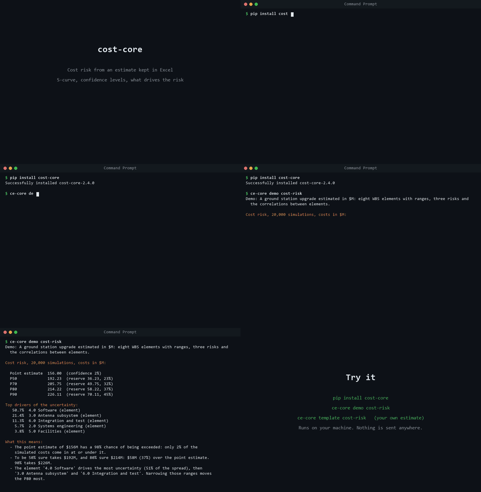
Try it on ready-made example workbooks: clone cost-core-starter and run python run_all.py.
Cost estimating, earned value and schedule analysis for defense and space
programs, as one Python package and one command, ce-core. Put your estimate
in Excel with a low, most likely and high for each WBS element, and it tells
you how likely the estimate is to be exceeded, what it takes to be 80% sure and
which elements drive the risk. It also forecasts a program's cost and finish
from its EVM data or an IPMDAR delivery, checks a Microsoft Project schedule
against the DCMA 14 points, runs joint cost and schedule confidence (JCL),
compares alternatives on life-cycle cost, chooses a portfolio within a budget,
fits learning curves and CERs, and reads real programs' unit costs out of
public SARs. Every result says what it means in plain words, and writes down
every assumption it made.
One tool where there are usually several. In most cost offices these jobs are split across commercial products and a lot of Excel: one tool for cost risk, another for schedule risk and JCL, another for schedule checks, and spreadsheets for EVM forecasts and AoAs. As far as I can find, cost-core is the first public Python package that does them together, on the same correlated Monte Carlo engine, with the same Excel-in, report-and-briefing-out workflow.
- Your data stays on your machine. Nothing is sent anywhere, there's no telemetry, and the only network call is the optional public SAR download.
- Free for noncommercial and government work, contractors included. See License for what's covered.
- Inputs are Excel workbooks, with an Instructions sheet and errors that name the sheet, row and column.
- Found a problem, or something unclear? Open an issue, with invented numbers only: never real program data or CUI.
Where it stands. It's young: first published in 2026, with one maintainer. About 1,200 automated tests and frozen reference results guard the numbers, and every release is checked against its source before it's announced. It hasn't yet been checked against published worked examples or reviewed by other estimators; that's the next step, and reports of where it disagrees with your own tools are the most useful feedback there is.
Start here
pip install "cost-core[plots]"   # the charts need the [plots] part
ce-core                          # what it can do, in plain English
ce-core demo cost-risk           # see it work on example data: no files needed
ce-core template cost-risk       # a workbook to fill in with your own estimate
ce-core open my_file.xlsx        # have a file already? it works out what it is
On Windows, ce-core open --send-to adds cost-core to the right-click
Send to menu: pick a file, send it, and the report opens in a folder
beside it.
If ce-core isn't found after installing (common on managed Windows PCs),
python -m cost_core does exactly the same. docs/getting-started.md
walks through each task from "what do I need" to "what does this tell me".
| I want to... | Try it | Then with my data |
|---|---|---|
| Forecast a program's final cost and finish from EVM | ce-core demo evm |
ce-core evm --data my_evm.xlsx or --ipmdar delivery.zip |
| How sure is my estimate, and what drives it (cost risk) | ce-core demo cost-risk |
ce-core cost-risk --data my_estimate.xlsx |
| Fit a CER from past programs and price a new one | ce-core demo cer |
ce-core cer --data my_cer.xlsx |
| Phase an estimate into a then-year budget by fiscal year | ce-core demo phase |
ce-core phase --data my_phase.xlsx |
| Check a schedule's logic (DCMA 14-point) | ce-core demo schedule |
ce-core schedule-check --mspdi my_schedule.xml |
| Know the chance of meeting a budget and a date (JCL) | ce-core demo jcl |
ce-core jcl --spec my_jcl.xlsx |
| Compare alternatives on life-cycle cost (AoA) | ce-core demo aoa |
ce-core aoa --spec my_aoa.xlsx |
| Choose which programs to fund within a budget | ce-core demo portfolio |
ce-core portfolio --spec my_portfolio.xlsx |
| Convert base-year and then-year dollars (with your index) | ce-core demo inflate |
ce-core inflate --index my_index.csv --data my_phasing.csv --from by2026 --to ty |
| Fit a learning curve to production lots | ce-core template lots |
ce-core fit-lots --csv my_lots.csv --dollar-year 2026 |
| See how real programs' unit costs grew | ce-core sar-panel --programs F-35 |
ce-core template <topic> writes the file to fill in for each one, and every
command answers --help. Every result also comes as one Excel workbook,
report.xlsx, with a plain-English summary, the tables, live charts and the
assumptions; in the EVM workbook the metrics are Excel formulas, so a
reviewer can click any CPI and see how it was made. And as a short
PowerPoint briefing, brief.pptx, that opens with the bottom line, then the
chart, the numbers behind it and the assumptions. The rest of this page shows each one.
Want a window instead of a terminal? lot-cost-model is a desktop tool for the lot cost engine: paste lots from Excel, fit, roll up a WBS and write the workbook, all through this library.
No proprietary data is committed to this repository. Examples and tests use invented numbers, apart from text from a few public Selected Acquisition Reports, which are U.S. government works.
Ready for the office
- Markings.
--marking "CUI"stamps exactly that text at the top and bottom of every slide and in the header and footer of every sheet. cost-core doesn't decide, check or validate markings; your organisation does. - Your slide master.
--template house.potx(or .pptx) buildsbrief.pptxon your organisation's template, using its "Title Slide" and "Title Only" layouts by name and scaling to its slide size, and says so if it has to fall back. - Set it once.
ce-core settings --writestarts ace-core.tomlfor the marking, the template, units, seed, iterations and the fiscal-year start (October by default). A flag on the command line always wins, then a setting in the input workbook or spec, then the file;ce-core settingsshows what's in effect and where each value came from. - Bug reports.
ce-core --aboutprints the versions to paste into an issue; nothing is sent anywhere.
What it does
| Module | Purpose |
|---|---|
cost_core.lotmodel |
The lot cost engine. Analogy lots in, estimate lots out. Fits LC / Rate / LC+Rate, selects on significance with an AICc tiebreak, and layers refits, influence, prediction intervals and buy risk on top. Carried over from the desktop tool in lot-cost-model, which runs on this code from its 3.0.0 rather than a copy of it |
cost_core.program |
WBS roll-up. Several elements, fitted, factor or amount, priced against one lot schedule and correlated into a programme estimate |
cost_core.lots |
Your own data. Units and cost per lot, in CSV or Excel. Runs the same three model engine, then layers the statistics on top |
cost_core.synth |
Seeded synthetic CSDR/SRDR generator: DD 1921, DD 1921-1, DD 1921-2, Cost and Hour Report (FlexFile), Quantity Data Report, SRDR (DD 2630), with realistic pathologies to clean |
cost_core.ingest |
ETL to one normalized long table: WBS crosswalk, base year normalization, resubmission dedup, loud validation gates, row level provenance |
cost_core.fitting |
Shared estimator: OLS, MUPE and ZMPE, with delta method prediction and confidence intervals |
cost_core.learning_curve |
Wright (cumulative average) and Crawford (unit) theories, rate breaks, prediction intervals |
cost_core.cer |
Parametric CERs, log log and linear, with leverage and influence diagnostics, extrapolation warnings, small sample guardrails |
cost_core.monte_carlo |
Correlated WBS level risk: Gaussian copula or Iman Conover, PSD repair, discrete risks, tornado, convergence |
cost_core.reporting |
S curve, tornado, cost improvement curve, CER diagnostics, and the assumptions log |
cost_core.evm |
Earned value. CPI, SPI, TCPI, the independent EACs and earned schedule from a spreadsheet or an IPMDAR delivery, the warning signs named, and the EAC and finish forecast as a calibrated range |
cost_core.aoa |
Analysis of alternatives. Life-cycle cost of each alternative in base-year, then-year and present-value dollars, compared under correlated uncertainty: P50, P80, the chance each is cheapest, cost-effectiveness and which are dominated |
cost_core.schedule |
Schedules, DCMA and JCL. Microsoft Project XML read in and checked against the DCMA 14 points; an activity network with uncertain durations, time-independent and time-dependent costs, a standing army and discrete risks, simulated jointly: the probability of meeting a budget and a date together, the 70% line, and how often each activity is critical |
cost_core.portfolio |
Which programs to fund. An integer program over candidates, funding options and yearly budgets, with mandatory programs, dependencies and exclusive alternatives; the marginal value of money by year, a value against budget frontier, and the chance the chosen portfolio breaks each year's budget |
cost_core.public |
Real programs. DoD's public Selected Acquisition Reports, 2010 to today, read into a program by year table of unit cost against the current and original baselines, with the source file and an arithmetic check behind every number |
Cost risk on an estimate kept in Excel
Most estimates already live in a workbook. Put each WBS element on a row with its point estimate and a low, most likely and high, add the discrete risks and which elements tend to overrun together, and run it:
ce-core demo cost-risk                                   # the invented example
ce-core template cost-risk                               # my_estimate.xlsx to fill in
ce-core cost-risk --data my_estimate.xlsx --out cost-risk/
It prints what the point estimate's confidence really is, what it takes to be
50%, 70%, 80% and 90% sure, and which elements and risks drive the spread, then
writes report.xlsx (S-curve, confidence table, drivers, elements, risks, the
correlation used and what ignoring it would cost), brief.pptx and the tables
as CSV. Only the Elements sheet is required; a CSV of elements works too.
Each element's range can be triangular (the default), PERT, uniform or
lognormal; a lognormal reads Low and High as the ends of an 80% range, which
is how ce-core cer hands over a CER's estimate. Pairs
of elements you don't list take the default correlation (0.3 unless the
Settings sheet says otherwise),
because leaving correlation out makes the P80 too low. The workbook never
leaves your machine.
It also shares the P80 out: how much of the reserve each element and risk needs, taken from the simulations whose total lands at the P80, so the shares add up to the P80 of the whole. Funding every element at its own P80 instead would overfund it, since percentiles don't add; the report shows by how much.
A CER from past programs
Put the programs you have data for on a Data sheet, one row each with its cost and its technical drivers (weight, power, lines of code), and the new programs on an Estimate sheet:
ce-core demo cer                                         # twelve invented radars
ce-core template cer                                     # my_cer.xlsx to fill in
ce-core cer --data my_cer.xlsx --out cer/
It fits the CER by OLS, MUPE and ZMPE side by side (log-log by default, or
linear), says what each coefficient means in cost ("doubling weight multiplies
the cost by 1.51"), and prices each new program with a prediction interval:
where one new program is expected to land, not the narrower interval on the
line itself. It names a driver whose effect can't be told apart from zero, a
program that pulls the fit more than the others, too few programs for the
drivers, and a new program outside the data, including one whose drivers are
each in range but whose combination isn't. A Use column leaves a program out
of the fit without deleting it, with a note saying why. report.xlsx has the
estimates, the methods compared, the coefficients with t-statistics and
p-values, the diagnostics and the data as fitted; brief.pptx and the CSVs
come with it.
Each estimate also comes as a row ready for a cost-risk Elements sheet: a lognormal whose Low and High are the prediction interval, so the CER's own uncertainty goes into the risk analysis instead of a range typed by hand.
From an estimate to a budget: phasing by fiscal year
Each line of the estimate gets an amount in base-year dollars, a start year, a number of years and a profile for how the money goes out:
ce-core demo phase                                       # five invented lines
ce-core template phase                                   # my_phase.xlsx to fill in
ce-core phase --data my_phase.xlsx --out phase/
The profiles are uniform, front or back loaded, a bell, a Rayleigh curve (the
usual shape of development spending, with its peak where you put it), or your
office's own percentages, one per year (10;30;40;20). Each line is inflated
to then-year dollars with the index on the Index sheet, or the one it names,
since RDT&E, procurement and O&M money each have their own. Out come the spend
by fiscal year in then-year and base-year dollars, by appropriation, what
inflation adds and the peak year, in report.xlsx, brief.pptx, a chart and
CSVs. The template's index is an invented 2% and says so; put your agency's
published indices in its place.
Earned value: where the program is heading
ce-core demo evm                                # the example below
ce-core evm --data my_evm.xlsx --units thousands --out evm/   # yours: ce-core template evm
ce-core template evm writes a spreadsheet laid out for it, holding the
example. Column names such as PV, EV, AC, "Planned Value" or "Month" are
recognised as well, so an export from another tool often reads as it is.
The data is the three numbers every EVM report carries, by period: BCWS, BCWP and ACWP, with the baseline running on past the status period and, optionally, the contractor's EAC and a control account column. From them come CV, SV, CPI, SPI, TCPI, the standard independent EACs, and earned schedule. SPI(t) and the IEAC(t) completion date are what to watch late in a program, since SPI drifts back to 1.0 as the last work is earned, however late.
Two things go further than the formulas:
- The EAC and the finish as a range. Every independent EAC formula
assumes some future efficiency, and they disagree by as much as the
program's performance has varied.
forecastruns the rest of the program many times on its own record: each simulated period earns schedule and spends at a pace and efficiency drawn, as a pair, from the periods so far, with runs of good and bad periods lasting as long as they did. The result is an EAC and a completion date with a P50 and a P80, their joint confidence, and where the contractor's EAC and each formula fall on it. On synthetic programs whose outcome is known, the P80 holds the true cost and finish 79 to 82% of the time (72 to 77% when performance is strongly persistent), and the test suite holds it to that. - The warning signs, stated. A contractor EAC whose TCPI is more than 0.10 above the CPI, one below every independent EAC, one that needs the CPI to recover more than 0.10 after 20% complete (Christensen's finding on DoD contracts), an SPI that has recovered while SPI(t) has not, and earned value beyond the budget.
- The monthly checks. Per control account: earned value or cost that went
backwards, cost with nothing earned, earned value with no cost, and an
account that's earned its whole budget but is still being charged, each
listed as a question to ask. And the accounts whose cumulative variance
breaks your thresholds (
--cv-pct,--sv-pct,--cv-dollars,--sv-dollars; 10% by default) and so owe a variance analysis report.
In the example, three invented control accounts at 32% complete, the contractor's EAC of $16.3M sits below the P1 of the forecast, whose P50 is $17.0M.
from cost_core.evm import EvmData, forecast
data = EvmData.read("cpr.csv")            # period, bcws, bcwp, acwp[, eac][, wbs]
data.flags()
forecast(data, seed=1).summary()
Straight from the IPMDAR (preview). The Contract Performance Dataset, the JSON tables contractors deliver under DI-MGMT-81861, reads directly:
ce-core evm --ipmdar cpd_2026_11.zip --out evm/
ce-core evm --ipmdar cpd_2026_*.zip --out evm/     # cumulative-only deliveries
Table and field names follow the CPD Data Exchange Instructions (March 2020). Work packages roll up into their control accounts, the baseline to complete and the contractor's estimate to complete come from their own tables, and the control accounts are reconciled against the PMB summary, with any gap stated. A dataset whose to-date values are time-phased holds the whole history. One that reports them only cumulative to date gives a single point, so pass the monthly deliveries together and the history is rebuilt from them, with any missing month named. A folder or ZIP of one JSON file per table and a single JSON file keyed by table name both read.
This reader is a preview. It follows the published Data Exchange Instructions and is tested on datasets written to them, but not yet on a real contractor delivery, and how the tables are packaged is still to be checked against the File Format Specification. Check the reconciliation note it prints against the delivery's own totals, and if a file does not read, please say so on the issue tracker (describe the file's layout; never attach the data). Until it is confirmed, a CSV export of BCWS, BCWP and ACWP by period is the dependable route.
Comparing alternatives: life-cycle cost for an AoA
An analysis of alternatives asks which way of meeting a need is worth its cost
over the whole life of the thing. Write the alternatives down in a workbook
(ce-core template aoa writes a complete one, with invented numbers) and run:
ce-core aoa --spec my_aoa.xlsx --out aoa/
        alternative        by        ty        pv       p50       p80  p_cheapest  effectiveness  cost_per_effectiveness     dominated_by
Keep current system  8,500.00 10,405.17  7,095.12  8,061.26  8,961.80        0.12           0.40               20,470.60 Upgrade in place
   Upgrade in place  7,460.00  8,849.00  6,416.03  7,062.21  7,556.72        0.83           0.62               11,472.89
    New development 13,570.00 17,349.43 11,075.61 12,430.58 13,413.85        0.00           0.90               13,916.31
     Buy commercial  8,930.00 10,899.62  7,534.64  8,017.60  8,415.43        0.06           0.55               14,637.96 Upgrade in place
Each alternative is a set of cost lines (development, procurement, operating and support, disposal), each phased by fiscal year in base-year dollars and carrying an uncertainty factor. Three things the module is careful about:
- Three kinds of money. Base-year dollars for building the estimate,
then-year dollars for the budget, and present value for the comparison.
Alternatives that spend at different times are compared on present value,
as OMB Circular A-94 requires, discounting constant dollars at a real
rate. There's no default rate: pass the current one from A-94 Appendix C
and it's recorded in
assumptions.json. Discounting then-year dollars at a real rate would count inflation twice, so the module never does. - Uncertainty decides rankings. Each alternative's lines are correlated
and simulated, so the answer is a distribution.
p_cheapestis the share of draws in which that alternative costs least, which says how firm a ranking is; two alternatives a few percent apart on point estimates are often a coin toss. - Cost is half the question. With effectiveness scores, the table gives cost per unit of effectiveness and names any alternative that another beats on both counts. In the example, buying commercial costs more than upgrading in place and does less, so it's off the frontier.
- Does the change pay for itself? Name the status quo (Status Quo on the
Settings sheet, or
--status-quo) and each alternative is measured against it, the way OMB A-94 and DoD's economic analysis guidance set out: the extra investment (RDT&E, procurement, MILCON) and the operating cost it saves (O&S, disposal) in present value, net savings, the savings-to-investment ratio, the discounted payback year, the undiscounted break-even year and the real IRR of the extra investment. Alternatives with different service lives are also compared on uniform annual cost, with a note saying so. In the example, upgrading in place repays its investment 1.6 times over by FY2039; new development doesn't pay back.
The spread on a line can come from history instead of judgement:
historical_growth takes the SAR panel above and returns each program's
latest unit cost growth against its original baseline, one observation per
program, and growth_factor turns it into a distribution a cost line can
carry.
from cost_core.aoa import CostLine, growth_factor, historical_growth, spread
history = historical_growth(panel.unit_cost, measure="APUC", max_quantity_change_pct=10)
line = CostLine("Production", "Procurement", spread(4200, 2032, 8), growth_factor(history))
Cost and schedule together: JCL
A cost S-curve says what money buys 70% confidence and nothing about when. For a project that carries a team for its whole life the two are one question, since every month of slip is a month of salaries. NASA budgets its major projects at the 70% joint cost and schedule confidence level (JCL): the probability of finishing at or under the cost and by the date.
ce-core demo jcl                          # the example below
ce-core jcl --spec my_jcl.xlsx --out jcl/   # yours, from: ce-core template jcl
The spec is an activity network in months: each activity has a most-likely duration with an uncertainty factor, its predecessors (finish-to-start, start-to-start, finish-to-finish or start-to-finish, with lags or leads), a time-independent cost (materials, a fixed-price contract) and a burn rate that costs more the longer it runs. The project carries a standing army, paid every month until it's done, and discrete risks that delay activities and add cost when they happen. The example, a small spacecraft with invented numbers, shows the three things a JCL analysis is for:
- The point estimate is almost never met. The plan of 43 months and $229M has under 1% joint confidence.
- Separate P70s aren't a 70% plan. Budgeting at the cost P70 and
scheduling at the schedule P70 reaches only 66% jointly, because the two
have to hold at once. The frontier gives the budget and date pairs that
really do reach 70%, and
jcl.pngdraws them over the cloud of simulated outcomes. - The long pole isn't always the critical path. The instrument is on the deterministic critical path and critical in 95% of runs; the criticality table is where management attention should go.
Schedule uncertainty in merging paths is what a deterministic plan misses most: two uncertain paths into one milestone finish later on average than either does alone (merge bias), so the critical path method is optimistic by construction. The simulation carries it; the test suite checks it.
From a Microsoft Project schedule
The network doesn't have to be retyped. Save the integrated master schedule from Microsoft Project as XML (MSPDI, which Primavera P6 and most other tools also export), check it's fit to simulate, then point a spec at it:
ce-core schedule-check --mspdi ims.xml --out check/
ce-core jcl --spec ims_jcl.json --out jcl/
schedule-check runs the DCMA 14-point assessment on the incomplete detail
tasks: missing logic, leads, lags, relationship types, hard constraints,
high and negative float, high duration, invalid dates, resources, missed
tasks, the critical path test, CPLI and BEI. It writes each check with its
threshold and every task that failed it, since a JCL run on dangling logic
and hard constraints is confident about nothing.
The spec names the file, with an uncertainty for every task and overrides for the ones you know more about; tasks are named by their name or UID:
{"mspdi": "ims.xml", "standing_army": 1.2,
 "duration_uncertainty": {"type": "triangular", "left": 0.9, "mode": 1.0, "right": 1.3},
 "per_task": {"Thermal vacuum test": {"type": "triangular", "left": 0.9, "mode": 1.0, "right": 2.0}},
 "risks": [{"name": "Late GFE", "probability": 0.3, "activities": ["Integrate payload"], "delay": 2}]}
Links keep their type and lag. Summary-task links move onto the tasks under
them. A task in progress keeps only its remaining work, so the simulation
runs from the status date. Each task's fixed cost stays fixed, and its
resource cost becomes a burn rate. Calendars and date constraints are not
modelled, and the run's assumptions.json says so, along with everything
else simplified on the way in.
Choosing a portfolio: which programs get funded
Moving money between programs is a capital budgeting problem, and the spreadsheet version of it is Excel Solver with a binary cell per program. Here it's a mixed-integer program solved with HiGHS through PuLP:
pip install "cost-core[optimize]"
ce-core portfolio --spec my_portfolio.xlsx --out portfolio/   # ce-core template portfolio
Each candidate has one or more funding options (full rate, minimum sustaining
rate, defer two years), each with a cost in every budget year and a value
score. The solver maximises value within every year's budget, funds the
mandatory programs, keeps dependencies ("integration needs the missile") and
picks at most one of each set of exclusive alternatives, which is what an AoA's
alternatives are: candidates_from_aoa turns an AoA result straight into them,
inflated to then-year dollars with the AoA's own index to sit against a
then-year budget (basis="by" keeps base-year dollars).
The optimum is where the analysis starts, and three more tables come with it:
- What an extra dollar is worth, by year.
marginal_valuere-solves with a little more money in one year at a time and says what it would buy. A year whose extra money buys nothing is where money can move from. - Value against budget.
frontiersolves at a range of budget levels, so the discussion can be about where value per dollar flattens. - Budget risk. An optimum on point estimates fills the budget almost
exactly, so cost growth breaks it.
budget_riskdraws correlated growth for each funded program (from SAR history viacost_core.aoa.growth_factor, or any distribution) and gives each year's chance of going over. In the example, the plan that fits on paper breaks its 2028 budget 94% of the time once costs grow the way the example's growth distribution says; planning to a growth factor (solve(..., cost_factor=1.15)) is the usual answer.
The solver is checked against brute force: on 40 random portfolios, every combination of options is enumerated and the integer program has to find the same best value.
Base-year and then-year dollars
ce-core demo inflate                  # an invented phased estimate, illustrative index
ce-core inflate --index my_index.csv --data my_phasing.csv --from by2026 --to ty
ce-core inflate --index my_index.csv --amount 100 --year 2030 --from by2026 --to ty
The index comes from you: your agency's published tables (the NASA New Start
Inflation Index, OSD inflation guidance), as index_name, fiscal_year, index_value. cost-core never carries those numbers itself;
ce-core template inflate shows the layout with an index that's plainly
marked as invented. Any year converts to any other, dates become fiscal years
(October start by default), every converted row keeps its original amount,
the factor and the index used, and a year outside the table is refused
rather than guessed.
Learning curves from production lots
Units and cost per lot is the whole input:
ce-core template lots
ce-core fit-lots --csv my_lots.csv --dollar-year 2026 --forecast "30,40" --out results/
It fits the curve, shows which lots it misses and by how much, puts an interval on the slope and forecasts the next buys with prediction intervals. docs/learning-curves.md covers the lot cost engine behind it (LC, Rate and LC+Rate, the WBS roll-up, the synthetic CSDR/SRDR pipeline), running it as a library, and the four things that quietly ruin a lot fit.
Real programs from public SARs
Every major defense program reports to Congress each year in a Selected Acquisition Report, and DoD releases them. Their unit cost pages are the longest public record of cost growth there is: what each program expected a unit to cost when it started, and what it expects now, in constant dollars.
pip install "cost-core[public]"
ce-core sar-panel --list-cycles
ce-core sar-panel --programs F-35 --out f35/
The second command reads the F-35's SARs from December 2010 to the FY 2027
budget and writes three files: unit_cost.csv (PAUC and APUC, baseline beside
current estimate, per subprogram and report), reports.csv (what was read and
what wasn't, and why) and checks.csv. Leave off --programs for all of them,
about a thousand reports, which takes an hour or two the first time and
seconds after, since every download is cached.
It works offline too, from a folder of SAR PDFs you already have
(ce-core sar-panel --dir path/to/sars). How the reports are read and checked,
and what the numbers mean: docs/public-sar-data.md.
Installation
Bringing it into a lab or a government office, behind a proxy, offline, or through a software approval review? docs/using-at-a-lab.md covers the licence question, the SBOM attached to every release, installing on a managed or air-gapped machine, and what touches the network.
Python 3.9 or higher. The distribution name is cost-core and the import name
is cost_core. It's on PyPI:
pip install "cost-core[plots]"
Leave off [plots] if you don't need the charts. To work on the code itself,
install from a clone instead:
python -m venv .venv && .venv/Scripts/activate && pip install -e ".[plots]"
That pulls in pandas, numpy, scipy and openpyxl, plus matplotlib for the
[plots] extra. Excel input and the workbooks the lot engine writes both need
openpyxl, so it's installed by default rather than as an extra. matplotlib is
the other way round: it draws the charts and nothing else, so installing without
the extra gives you the whole engine, the CERs, the risk simulation and the Excel
workbooks, and anything that draws a PNG tells you to add [plots] when you
reach it.
numpy and scipy carry upper bounds so the published numbers reproduce exactly; docs/development.md explains why, and how to run the tests.
How the numbers are made
The method choices are argued for, not just made: docs/methods.md explains why MUPE and ZMPE sit beside OLS, why intervals are prediction intervals and not confidence intervals, why correlation matters, why the fit is judged on standard error and CV rather than R², and why Wright and Crawford are different theories.
Mapping to the GAO Cost Estimating and Assessment Guide
ce-core full-run and fit-lots --out write an ASSUMPTIONS.md organized
around the four characteristics of a reliable estimate; the other commands keep
their settings on the Assumptions sheet of report.xlsx.
| Characteristic | How this library addresses it |
|---|---|
| Comprehensive | All six report shapes ingested. Recurring and nonrecurring cost, five functional categories and discrete risks all modeled. The WBS crosswalk surfaces unmatched elements rather than dropping them |
| Well-documented | Row level provenance from every output number back to its source submission. The crosswalk and inflation index are persisted artifacts, not inline logic. The assumptions log separates what was measured from what was assumed, and counts the assumptions |
| Accurate | Validation gates reconcile row counts and dollar totals within and across reports, and fail the run when they disagree. Retransformation bias is measured and corrected. Estimating methods are compared rather than assumed |
| Credible | Prediction intervals on every forecast. Leverage and influence diagnostics on the CER. Extrapolation flagged, including hidden extrapolation. The correlation assumption's effect quantified against independence. P80 convergence checked |
License
Versions 1.0.0 and 1.0.1 were released under the Apache License 2.0 and stay that way. Everything after them is under the PolyForm Noncommercial License 1.0.0. In plain terms:
- Free for any noncommercial purpose: personal study, research, teaching, hobby projects.
- Free for schools and universities, public research organizations, government institutions, charities, and public safety, health and environmental organizations, whatever their funding. A government cost office or a university research lab can use it as it stands.
- Free for government work, including for contractors. An additional permission lets anyone, commercial companies included, use it for work done for or under a U.S. government contract, subcontract at any tier, grant or other agreement: prime contractors running their own EVM and schedules, support contractors in a government cost office, and the proposals and cost estimates for such work.
- Other commercial use needs a license from the author. That includes selling the software, building it into a product or hosted service offered beyond a government agreement, and work for commercial customers. A deliverable a government contract calls for, delivered under it, counts as government work. Ask through the issue tracker.
Anyone who passes on a copy of any part of it has to pass on the license terms
and the Required Notice: line in NOTICE with it. This is a plain
summary; LICENSE and LICENSE-GOVERNMENT-WORK.md are what govern.
1 maintainer

Metadata
1 maintainer
Release files for cost-core 2.7.0
For a detailed explanation of source distributions (sdists) and built distributions (wheels), please see the package formats documentation.
Source distribution (sdist)
| File | Size | Uploaded | |
|---|---|---|---|
| cost_core-2.7.0.tar.gz | 1.9 MB | Details |
Built distribution (wheel)
| File | Interpreter | ABI | Platform | Reset |
|---|---|---|---|---|
| cost_core-2.7.0-py3-none-any.whl | Python 3 | none | any | Details |
Total release size: 2.3 MB
Release files / cost_core-2.7.0.tar.gz
| Download URL | cost_core-2.7.0.tar.gz |
|---|---|
| Size | 1.9 MB |
| Tags | Source |
|
SHA-256 checksum How to use checksums |
902fd263c8831d8bf68a76dbd13e906d64116e731015e90ec3f7a0ba9fc61a0f
|
|
BLAKE2b-256 checksum How to use checksums |
4f5928ac6079785af7fcb4429ce3d3d07f6d27c54bfcf2e35c57f8abe23efa01
|
| Upload date | |
|
Uploaded using Trusted Publishing? What is trusted publishing? |
Yes |
| Uploaded via |
twine/7.0.0 CPython/3.13.14
|
Provenance
Provenance describes where a file came from. On PyPI, provenance is shared via attestations, which provide a verifiable record of the build or publishing details. View details, limitations and caveats.


PyPI Publish Attestation
PyPI verified that this artifact, at this checksum, originated from the publisher listed below.
Signed by GitHub Actions, verified by PyPI on Oct 1, 2026.
Transparency logRelease files / cost_core-2.7.0-py3-none-any.whl
| Download URL | cost_core-2.7.0-py3-none-any.whl |
|---|---|
| Size | 453.5 kB |
| Tags | Python 3 |
|
SHA-256 checksum How to use checksums |
9144919b3f56713f098a1b5df7e9d584ad46d29f5a9234ba430d95173767d755
|
|
BLAKE2b-256 checksum How to use checksums |
3ac9b90ee1e5f1809dd57025c35d25b76fe46f583eed42be93a83452c06fd334
|
| Upload date | |
|
Uploaded using Trusted Publishing? What is trusted publishing? |
Yes |
| Uploaded via |
twine/7.0.0 CPython/3.13.14
|
Provenance
Provenance describes where a file came from. On PyPI, provenance is shared via attestations, which provide a verifiable record of the build or publishing details. View details, limitations and caveats.
PyPI Publish Attestation
PyPI verified that this artifact, at this checksum, originated from the publisher listed below.
Signed by GitHub Actions, verified by PyPI on Oct 1, 2026.
Transparency log













