





A Python toolkit for producing publication-quality microeconomics diagrams. Define utility functions declaratively, solve for consumer equilibria, and export figures as PNG, PDF, SVG, or pure TikZ — all in a few lines of code.
Installation
pip install econ-viz
Requires Python 3.10 or later.
Quick Start
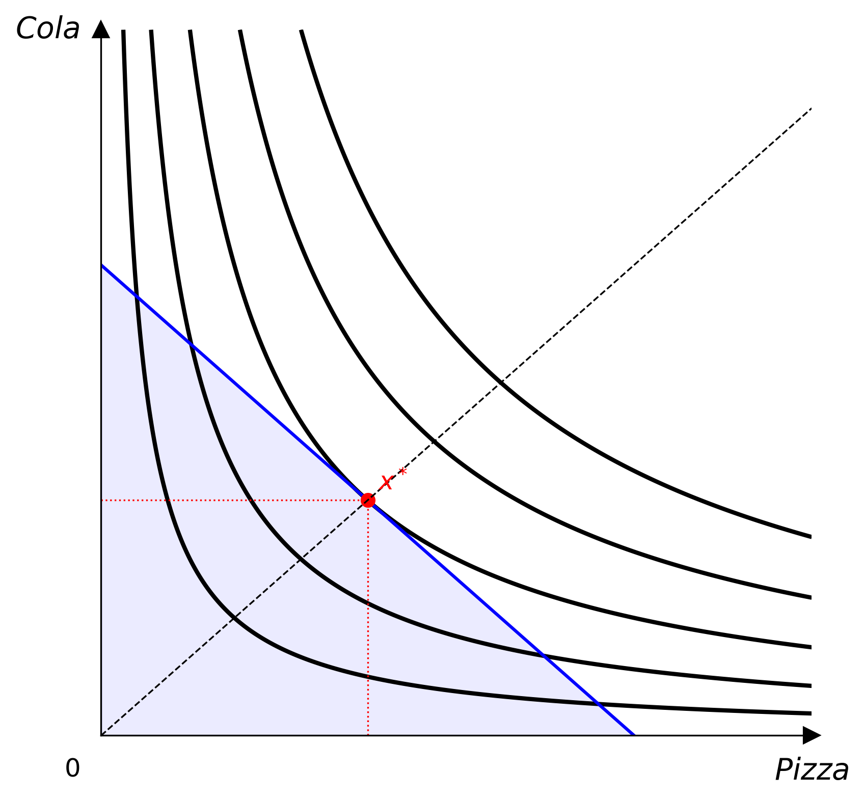
from econ_viz import Canvas, levels, solve
from econ_viz.models import CobbDouglas

model = CobbDouglas(alpha=0.5, beta=0.5)
eq    = solve(model, px=2.0, py=3.0, income=30.0)
lvls  = levels.around(eq.utility, n=5)

cvs = Canvas(x_max=20, y_max=15, x_label="x", y_label="y",
             title="Cobb-Douglas  $x^{0.5} y^{0.5}$")
cvs.add_utility(model, levels=lvls)
cvs.add_budget(2.0, 3.0, 30.0, fill=True)
cvs.add_equilibrium(eq, show_ray=True)
cvs.save("cobb_douglas.png")
TikZ export writes a standalone LaTeX document with only TikZ drawing commands:
cvs.save("cobb_douglas.tex", tikz_scale=0.0125)
The default TikZ scale maps a 6 inch wide Matplotlib figure to about 7.5 cm.
Notebook
The project ships with an interactive playground notebook:
notebook/econ-viz Playground.ipynb
Download it and open it in Jupyter, VS Code, or Colab. The first code cell upgrades econ-viz from PyPI for fresh runtimes.
Highlights
- Built-in models: Cobb-Douglas, Leontief, Perfect Substitutes, CES, Satiation, Quasi-Linear, Stone-Geary, and Translog
- Solver support for interior, kink, boundary, and corner solutions
- Closed-form demand helpers with
solution_tex(...) - Comparative tools including
comparative_statics(...)andslutsky_matrix(...) - Multi-panel
Figurelayouts,PricePath/IncomePath, and linkedDemandDiagram - CLI support for plotting and closed-form demand output
- Color-blind-friendly default palette (
themes.COLORBLIND_CYCLE_RGB) sourced from thriveth/8560036, with related citation at DOI:10.1080/00220485.1996.10844911
Additional Tools
Axis labels can be placed around their arrowheads, and each axis can use its own arrowhead style and line style (solid, dashed, dotted, or dashdot):
from econ_viz import ArrowStyle, Canvas, LabelPosition, LineStyle

canvas = Canvas(
    x_label_pos=LabelPosition.TOP,
    y_label_pos=LabelPosition.RIGHT,
    x_arrow_style=ArrowStyle.SIMPLE,
    y_arrow_style=ArrowStyle.WEDGE,
    x_line_style=LineStyle.DASHED,
)
Every line can be restyled with a Stroke: width, line style, colour, and an
arrowhead at its end. Fields you leave out keep the theme default (see the
*_stroke defaults on Theme, such as theme.budget_stroke):
from econ_viz import ArrowStyle, Stroke

canvas = Canvas(axis_stroke=Stroke(width=1.4, arrow=ArrowStyle.SIMPLE))
canvas.add_budget(2, 3, 30, stroke=Stroke(width=3, style="dashed"))
canvas.add_equilibrium(eq, drop_stroke=Stroke(style="dashdot"))
canvas.add_ray(0.5, stroke=Stroke(arrow=ArrowStyle.TRIANGLE))
add_utility, add_path, add_decomposition, DemandDiagram, and
EdgeworthBox take one *_stroke argument per kind of line they draw.
Stroke is the preferred way to style lines; the separate color,
linewidth, and linestyle arguments still work as shorthand and draw the
same thing.
Point markers work the same way with Marker (colour, size, and shape);
fields you leave out keep the theme default, such as theme.eq_marker:
from econ_viz import Marker

canvas.add_equilibrium(eq, marker=Marker(shape="s", size=8))
canvas.add_point(12, 2, label="A", marker=Marker(color="black", shape="D"))
canvas.add_decomposition(dec, point_marker=Marker(shape="^"))
Point labels take a Label (text, position, offset, colour, size, and
visibility) wherever a plain string worked. A label follows its point's
Marker colour unless it sets its own:
from econ_viz import Label

canvas.add_equilibrium(eq, label=Label(position="bottom-left", offset=8))
canvas.add_point(12, 2, label=Label(text="A", position="left", fontsize=14))
canvas.add_utility(u, levels=3, ic_label=Label(text="U={:.1f}", position="top"))
canvas.add_decomposition(dec, point_label=Label(visible=False))  # hide A, B, C
Shade the budget set with fill=True, or pass a Fill for a colour and
opacity of its own (default theme.budget_fill, coloured like the line):
from econ_viz import Fill

canvas.add_budget(2, 3, 30, color="black", fill=Fill(color="lightgrey", alpha=0.4))
Each axis's label, label position, and stroke fit in one Axis, accepted by
Canvas, Figure, DemandDiagram, and EdgeworthBox. x_label,
x_label_pos, and x_axis_stroke stay as shorthand; an Axis field wins
when both are set:
from econ_viz import Axis, Stroke

canvas = Canvas(
    x_axis=Axis(label="x_1", label_position="bottom", stroke=Stroke(width=1.2)),
    y_axis=Axis(label="x_2"),
)
Set a font for one canvas or a whole multi-panel figure without touching
Matplotlib's global settings. Pass a family name, a generic family such as
"serif", or a fallback list:
from econ_viz import Figure, Layout

canvas = Canvas(font=["Times New Roman", "serif"], math_font="stix")
figure = Figure(Layout.SIDE_BY_SIDE, font="serif", math_font="stix")
font applies to titles, axis labels, annotations, curve labels, and legends.
Math text, including the default axis labels, uses math_font: "stix"
(Times-like), "cm" (Computer Modern), "dejavuserif", "dejavusans", or
"stixsans". An unavailable font raises
InvalidParameterError. TikZ output uses the LaTeX document's fonts, so only
generic families are mapped (serif → \rmfamily, monospace → \ttfamily).
Closed-form Marshallian demand in TeX:
from econ_viz import solution_tex
from econ_viz.models import CobbDouglas

tex = solution_tex(CobbDouglas(alpha=0.4, beta=0.6))
Slutsky matrix:
from econ_viz import slutsky_matrix
from econ_viz.models import CobbDouglas

S = slutsky_matrix(CobbDouglas(alpha=0.4, beta=0.6), px=2.0, py=3.0, income=60.0)
# S.s_xx, S.s_xy, S.s_yx, S.s_yy
CLI
econ-viz --version
econ-viz help
econ-viz models
econ-viz solve-tex --model cobb-douglas --symbolic-params
Plotting example:
econ-viz plot --model cobb-douglas --alpha 0.5 --beta 0.5 \
              --px 2 --py 3 --income 30 \
              --fill --show-ray \
              --output cobb_douglas.png
Documentation
Full documentation lives at econ-viz.org.
License
MIT © Anthony Sung
1 maintainer

Release files for econ-viz 1.8.0
For a detailed explanation of source distributions (sdists) and built distributions (wheels), please see the package formats documentation.
Source distribution (sdist)
| File | Size | Uploaded | |
|---|---|---|---|
| econ_viz-1.8.0.tar.gz | 88.0 kB | Details |
Built distribution (wheel)
| File | Interpreter | ABI | Platform | Reset |
|---|---|---|---|---|
| econ_viz-1.8.0-py3-none-any.whl | Python 3 | none | any | Details |
Total release size: 209.3 kB
Release files / econ_viz-1.8.0.tar.gz
| Download URL | econ_viz-1.8.0.tar.gz |
|---|---|
| Size | 88.0 kB |
| Tags | Source |
|
SHA-256 checksum How to use checksums |
0349768fe3a8fabee6e5f1af3d564a14db8eac60fad3b87ed24ad7bb037ce064
|
|
BLAKE2b-256 checksum How to use checksums |
b693717decc1cb7b693e5be378d8e98beae4c07f46da267045dab7bdc37e77d0
|
| Upload date | |
|
Uploaded using Trusted Publishing? What is trusted publishing? |
Yes |
| Uploaded via |
twine/7.0.0 CPython/3.13.14
|
Provenance
Provenance describes where a file came from. On PyPI, provenance is shared via attestations, which provide a verifiable record of the build or publishing details. View details, limitations and caveats.


PyPI Publish Attestation
PyPI verified that this artifact, at this checksum, originated from the publisher listed below.
Signed by GitHub Actions, verified by PyPI on Sep 26, 2026.
Transparency logRelease files / econ_viz-1.8.0-py3-none-any.whl
| Download URL | econ_viz-1.8.0-py3-none-any.whl |
|---|---|
| Size | 121.2 kB |
| Tags | Python 3 |
|
SHA-256 checksum How to use checksums |
7f9d22dbb622df547b95081ac2d89ab5d4cbb79c6bc08d7c645d760521476ab2
|
|
BLAKE2b-256 checksum How to use checksums |
fde5fbeb1a7f7e18518173edf56365901682efe08080c277cf325a41dad0aa7a
|
| Upload date | |
|
Uploaded using Trusted Publishing? What is trusted publishing? |
Yes |
| Uploaded via |
twine/7.0.0 CPython/3.13.14
|
Provenance
Provenance describes where a file came from. On PyPI, provenance is shared via attestations, which provide a verifiable record of the build or publishing details. View details, limitations and caveats.
PyPI Publish Attestation
PyPI verified that this artifact, at this checksum, originated from the publisher listed below.
Signed by GitHub Actions, verified by PyPI on Sep 26, 2026.
Transparency log













