



Free Energy Landscape Analysis
Builds the free energy landscape of a molecular dynamics simulation from two collective variables, finds its metastable states, and gives you a representative frame for each one.
Input is two text files of frame value. Output is five figures, an animation and two tables.
Install
pip install free-energy-landscape
Requires Python 3.10 or newer; tested through 3.14.
Usage
free_energy_landscape cv1.txt cv2.txt --names "CV1 (Angle)" "CV2 (Distance)"
Every figure below was produced by that same command run on the two files in inputs/:
free_energy_landscape inputs/proj1Out.txt inputs/proj2Out.txt --names "CV1 (Angle)" "CV2 (Distance)"
Everything else is default. The run is deterministic — no seed, no k, no initialisation — so the
same input gives byte-identical output on any machine and for any number of cores.
Each CV file is two columns, frame index and CV value. Both must describe the same trajectory: same number of rows, same frame index on every row. See docs/OPTIONS.md for every command-line flag.
Theoretical background
The free energy landscape is a conceptual and computational tool used to understand the energetics and dynamics of molecular systems. It is particularly useful for interpreting molecular dynamics simulations, where it condenses a trajectory of millions of coordinates into the energetics of the processes the system actually undergoes: protein folding, chemical reactions, and phase transitions.
Collective variables (CVs) are the coordinates that make this possible. They reduce the full set of atomic coordinates to the few degrees of freedom that matter — a principal component, a distance, an angle, a dihedral — so the state of the system can be described by a handful of numbers.
How it works
1. Density. A Gaussian kernel density estimate turns the frames, one point each in the 2D CV
space, into a smooth probability density f on a regular grid. One kernel is fitted over the whole
trajectory; parallelism splits only its evaluation.
2. Free energy. Boltzmann inversion, shifted so the global minimum sits at zero:
G = -kB · T · ln f then G <- G - min G
3. Sampling mask. A kernel estimate returns a number even where no frame exists, and that number is extrapolation, not measurement. A cell counts as sampled only when the estimate expects at least one frame inside it:
f(cell) · area(cell) · N >= mask_min_count (default 1 frame)
The rest is left out of the analysis and of the colour scale.
4. Steepest descent. Each cell points at its lowest neighbour among the eight surrounding it, or at itself if none is lower. Following those pointers to their fixed point gives the local minimum each cell drains into — its basin of attraction, which is the operational definition of a metastable state.
5. Saddles. Neighbouring basins meet along a ridge. The saddle between them is the lowest point of that ridge, the cheapest way across:
saddle(A,B) =   min      max( G(x), G(y) )
              x in A
              y in B
              adjacent
6. Depth. How far a basin must climb to escape — its topological persistence:
depth(A) =  min saddle(A,B)  -  min  G(x)
             B                 x in A
7. Merging. Basins shallower than the cut are absorbed by the neighbour across their lowest
saddle. The cut is chosen at the largest step in the sorted depths, where real structure and
estimator ripple separate, and never exceeds kB·T. What it chose and what it merged is printed
on every run:
Watershed found 12 local minima; --basin_min_depth 1.01 kJ/mol (auto) merged 7 of them.
Barrier depths (deepest first): 2.10, 1.81, 1.59, 1.43, 1.41, 0.61, 0.47, 0.27, 0.17, ...
Largest step is 1.41 -> 0.61 kJ/mol: --basin_min_depth between them keeps 6 basins.
8. Representatives. Each frame inherits the basin of its cell. The representative of a basin is the frame of lowest free energy inside it — an actual conformation, ready to extract from the trajectory.
Full derivation, a worked one-dimensional example, and why DBSCAN is not used: METHOD.md.
Result
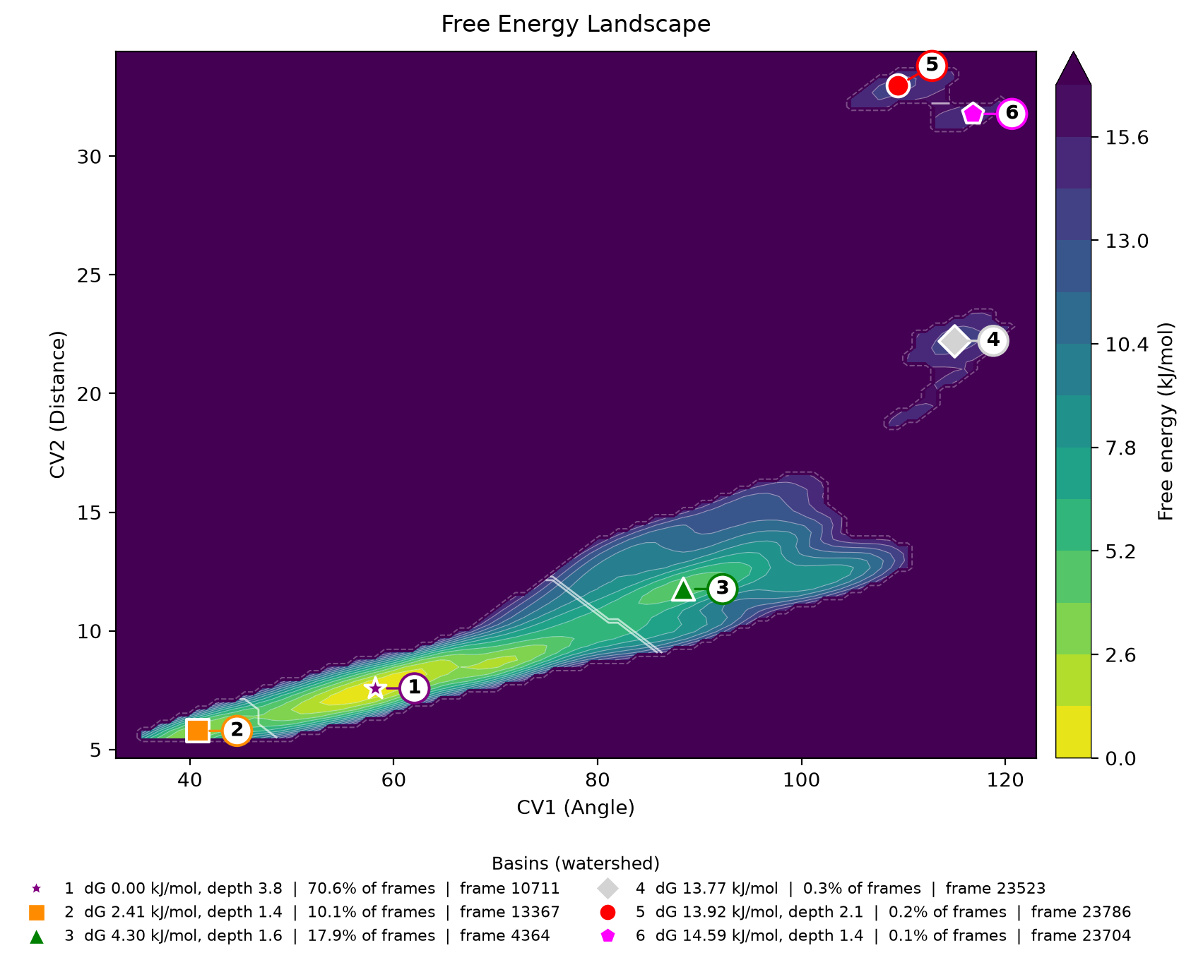
The two collective variables combined. Bright is low energy, dark is high; the region beyond the dashed line was never sampled, so no energy is claimed there. White lines are the watershed ridges separating basins, and each numbered callout marks a basin minimum — the legend gives its depth, its share of the trajectory, and its representative frame.
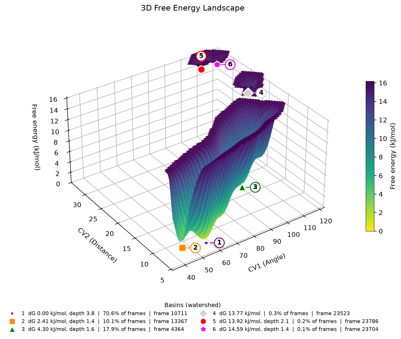
The same surface as relief, which makes the depth of each basin and the height of the barriers between them directly comparable.
The run also writes the free energy profile and distribution of each CV separately, both CVs against frame number, and a rotating animation of the 3D surface — all six are described in docs/FIGURES.md.
Tables
basins.tsv — one row per metastable state:
  #        CV1        CV2       dG    depth   frames    pop%  rep frame
-----------------------------------------------------------------------
  1     58.181      7.578     0.00     3.82    36447   70.58      10711
  2     40.777      5.786     2.41     1.41     5201   10.07      13367
  3     88.408     11.761     4.30     1.59     9263   17.94       4364
  4    114.971     22.219    13.77        -      164    0.32      23523
  5    109.475     32.975    13.92     2.10       98    0.19      23786
  6    116.803     31.780    14.59     1.43       43    0.08      23704
dG is the basin minimum relative to the global minimum, depth how far it must climb to reach a neighbour, pop% its share of the trajectory, and rep frame the conformation to extract. A dash under depth means the basin has no neighbour: it sits on its own island of sampled space.
discrete_values_energy_frames.tsv — every frame with its energy and basin id, sorted by energy.
Documentation
- docs/METHOD.md — the method in full, with a worked example and the reasoning behind each choice
- docs/FIGURES.md — all six figures, with what each axis means
- docs/OPTIONS.md — every command-line flag, input format, output files
- CHANGELOG.md — what changed in 2.0.0 and why results differ from 1.x
Citation
10.5281/zenodo.10689689 — the concept DOI, which always resolves to the latest release. Zenodo also mints a DOI per version if you need to cite the exact one you ran.
1 maintainer

Download files
Download the file for your platform. If you're not sure which to choose, learn more about installing packages.
Source Distribution
Built Distribution
Filter files by name, interpreter, ABI, and platform.
If you're not sure about the file name format, learn more about wheel file names.
Copy a direct link to the current filters
File details
Details for the file free_energy_landscape-2.0.0.tar.gz.
File metadata
- Download URL: free_energy_landscape-2.0.0.tar.gz
- Upload date:
- Size: 38.3 kB
- Tags: Source
- Uploaded using Trusted Publishing? No
- Uploaded via:
twine/7.0.0 CPython/3.14.6
File hashes
| Algorithm | Hash digest | |
|---|---|---|
| SHA256 |
ecab6eb8fff0185418fe0e694d47c43750959b45683329d487266c97fc8ad9e9
|
|
| MD5 |
64d357c08e66e4bae17fb9c283c484f6
|
|
| BLAKE2b-256 |
763d44a58d694407d30d20b659fbf52d3f8603a89952584d6dcad18776571334
|
File details
Details for the file free_energy_landscape-2.0.0-py3-none-any.whl.
File metadata
- Download URL: free_energy_landscape-2.0.0-py3-none-any.whl
- Upload date:
- Size: 28.4 kB
- Tags: Python 3
- Uploaded using Trusted Publishing? No
- Uploaded via:
twine/7.0.0 CPython/3.14.6
File hashes
| Algorithm | Hash digest | |
|---|---|---|
| SHA256 |
4a5422dca24a0fe08b71b34b573a40be54150bfed13db0fece7bf85740b22396
|
|
| MD5 |
62a8e847545eb192c915d334086ddefb
|
|
| BLAKE2b-256 |
c15ffff4e4b81ed898b7441ba98f735f7f781e46467300772059d27e751e3463
|







