Imaging Atmospheric Cherenkov Telescopes simulation

Project description
iactsim: Imaging Atmospheric Cherenkov Telescope Simulation


Overview
iactsim is a Python package designed for simulating the response of Imaging Atmospheric Cherenkov Telescopes (IACTs). It exploits the computational power of GPUs to accelerate computationally intensive tasks such as ray-tracing and SiPM response simulation. This project aims to provide a fast, flexible, and user-friendly simulation framework for IACT performance studies, instrument design and data analysis.
Features
- GPU-accelerated ray-tracing
- GPU-accelerated camera response
- Runtime configuration
- And more...
Installation
Prerequisites
-
Python: >=3.11
-
NVIDIA HPC SDK:
iactsimrequires the NVIDIA HPC Software Development Kit (SDK) to compile CUDA kernels -
CuPy:
iactsimutilizes CuPy for GPU offloading -
CMake: >=3.15
-
A C++ compiler:
gccornvcc
Installation Instructions
It is recommended to use a virtual environment. For example, using mamba:
mamba create -n simenv python=3.13
mamba activate simenv
You need a compiler for the C++ part. If you use HPC SDK compilers, as recommended here, you can use them
with module load nvhpc before calling pip. You can choose gcc or nvcc appending -C cmake.args="-DCMAKE_CXX_COMPILER=<compiler_name>" to the install command, replacing <compiler_name> with the actual compiler name.
(PyPI)
iactsim source archive is available on PyPI:
pip install iactsim -v
(dev)
-
Clone the repository:
git clone https://gitlab.com/davide.mollica/iactsim.git
-
Move inside the cloned folder and install
iactsimfrom source:cd iactsim python -m pip install . -v
For developers
You can install package locally without recompiling the C++ part (if has not changed) with the following
python -m pip install --no-build-isolation -e .
To do so, you need to have all the dependencies installed in your system:
pip install scikit-build-core pybind11 "setuptools_scm[toml]>=8.0" cmake ninja
zlib
For the C++ part, by deafult zlib-ng (zlib data compression library for the next generation systems) will be used (cmake will clone the repo automatically). If you have to use zlib or you do not need to decompress gzip CORSIKA files, you can append -C cmake.args="-DUSE_ZLIBNG=OFF" to the install command.
NVHPC
Configure the enviroment to use HPC SDK compilers (you can download HPC SDK from the NVIDIA website). We suggest to use Environment Modules to handle SDK configuration and then define NVCC and CUDA_PATH enviromental variables:
module load nvhpc
export NVCC=$NVHPC_ROOT/compilers/bin/nvcc
export CUDA_PATH=$NVHPC_ROOT/cuda
With conda/mamba enviroments you can use the provided configuration script configure_conda_env
mamba activate simenv
configure_conda_env simenv
mamba deactivate
This adds an activation script and a deactivation script to the simenv enviroment that will automatically handle the configuration when it is activated or deactivated.
Install CuPy
pip install cupy-cuda<XXX>
Replace with your CUDA version (e.g., cupy-cuda12x).
For more detailed instructions on installing CuPy, refer to the CuPy documentation.
Conda virtual environments and Jupyter
If you want to run Jupyter Notebook or JupyterLab from a different environment (usually the base environment) and access the new one, do the following:
-
Install nb_conda_kernels in the base environment:
mamba deactivate
mamba install nb_conda_kernels
-
Make sure
ipykernelis installed in the new virtual environmentmamba install -n simenv ipykernel
Now you can find the new environment kernel in JupyterLab/Notebook kernels list (Kernel->Change kernel in the menu bar).
In order to let the tqdm progress bar work properly, install ipywidgets following the installation guide.
Usage
Optical system definition
import iactsim
import matplotlib.pyplot as plt
plt.style.use('iactsim.iactsim')
# Spherical mirror
mirror_curvature_radius = 20000
plate_scale = mirror_curvature_radius/57.296/2.
mirror = iactsim.optics.SphericalSurface(
half_aperture=10000.,
curvature=1./mirror_curvature_radius,
position=(0,0,0),
surface_type=iactsim.optics.SurfaceType.REFLECTIVE_FRONT, # reflective in the pointing direction
name = 'Mirror'
)
# Flat focal surface (5deg hexagon)
focal_plane = iactsim.optics.FlatSurface(
half_aperture = 5*plate_scale,
position = (0,0,0.5*mirror_curvature_radius),
aperture_shape = iactsim.optics.ApertureShape.HEXAGONAL,
surface_type=iactsim.optics.SurfaceType.SENSITIVE_BACK, # sensitive surface opposite to the pointing direction
name = 'Focal Plane'
)
# Optical system
os = iactsim.optics.OpticalSystem(surfaces=[focal_plane, mirror], name='TEST-OS')
# Telescope position
pos = (0,0,0)
# Telescope pointing (alt,az)
poi = (0.,0.)
# IACT
telescope = iactsim.IACT(os, position=pos, pointing=poi)
# Copy data to the device
telescope.cuda_init()
# Photon source initialized on-axis
source = iactsim.optics.sources.Source(telescope)
source.positions.radial_uniformity = False
source.positions.random = False
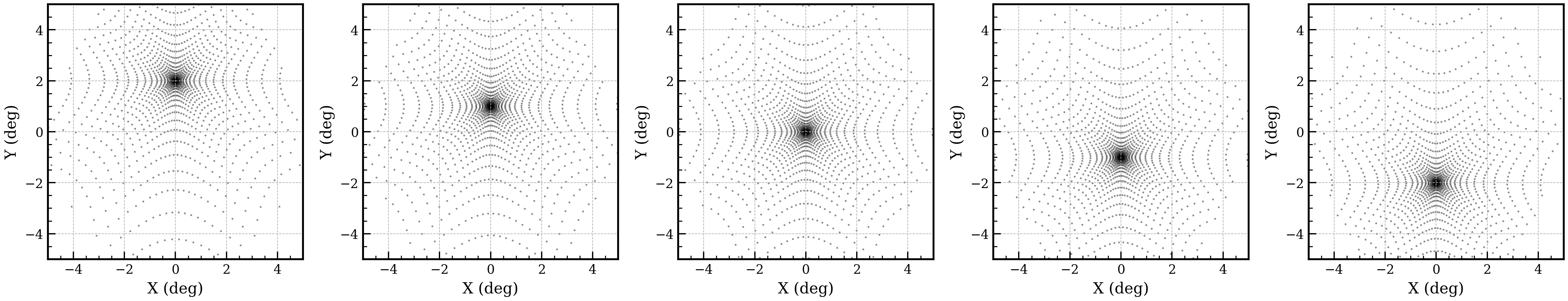
# Plot spot diagram at different off-axis angles
n_plots = 5
fig, axes = plt.subplots(1,n_plots,figsize=(3.5*n_plots,3.5))
source.directions.altitude -= 2.
for ax in axes:
# Adjust photon position to match the mirror position
source.set_target('Mirror')
# Generate photons
ps, vs, wls, ts = source.generate(10000)
# Perform ray-tracing
telescope.trace_photons(ps, vs, wls, ts)
# Plot spot diagram
iactsim.visualization.scatter(ps, s=0.2, ax=ax, color='black', alpha=0.5, scale=plate_scale)
ax.set_xlabel('X (deg)')
ax.set_ylabel('Y (deg)')
ax.grid(ls='--')
# Move the source
source.directions.altitude += 1. # degree
plt.tight_layout()
plt.show()
Mirror segmentation
The following code provides an example of how to segment a surface (AsphericalSurface, SphericalSurface or FlatSurface) starting from a mother surface (in this case mirror).
Note that each segment is an independent surface and does not need a mother surface, which is used here simply for convenience.
import numpy as np
# List of segments
segments = []
# Segment ID
k = 0
# Segments on a 10X10 grid, 80 total
n = 10
segment_distance = 2*mirror.half_aperture / (n+3)
for i in range(n+3):
for j in range(n+3):
offset = [
-mirror.half_aperture+segment_distance*i,
-mirror.half_aperture+segment_distance*j
]
r_segment = np.sqrt(offset[0]**2+offset[1]**2)
# Do not create segments outside the original mirror aperture
if r_segment > mirror.half_aperture-segment_distance*np.sqrt(2):
continue
# Ideal segment position
segment_position = [
offset[0],
offset[1],
mirror.sagitta(r_segment),
]
# Create the surface
segment = iactsim.optics.SphericalSurface(
curvature=mirror.curvature,
half_aperture=0.45*segment_distance,
position=segment_position,
surface_type=mirror.type,
name = f'Segment-{k}',
aperture_shape=iactsim.optics.ApertureShape.SQUARE,
tilt_angles=np.random.normal(0,1,3), # Big random dispersion
scattering_dispersion=0.05
)
# Specify the segment offset
# When a segment is created in this way:
# - it will be oriented with the same surface normal
# of the mother surface at the specified offset
# - `tilt_angles` attribute will define a deviation from this orientation.
segment.offset = offset
segments.append(segment)
k += 1
# Optical system
segmented_os = iactsim.optics.OpticalSystem(
surfaces=[focal_plane, *segments],
name='SEGMENTED-TEST-OS'
)
# IACT
segmented_telescope = iactsim.IACT(segmented_os, position=pos, pointing=poi)
segmented_telescope.cuda_init()
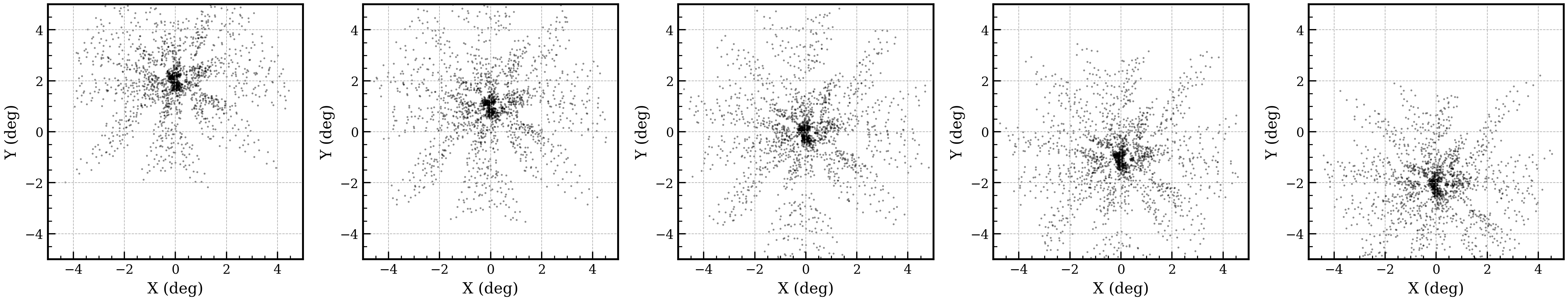
# Plot spot diagram at different off-axis angles
n_plots = 5
fig, axes = plt.subplots(1,n_plots,figsize=(3.5*n_plots,3.5))
# Photon source initialized on-axis
source = iactsim.optics.sources.Source(segmented_telescope)
source.positions.radial_uniformity = False
source.positions.random = False
source.positions.r_max = mirror.half_aperture*1.5
source.directions.altitude -= 2.
for ax in axes:
# Adjust photon position to match the mirror position
source.set_target()
# Generate photons
ps, vs, wls, ts = source.generate(10000)
# Perform ray-tracing
segmented_telescope.trace_photons(ps, vs, wls, ts)
# Plot spot diagram
iactsim.visualization.scatter(ps, s=0.2, ax=ax, color='black', alpha=0.5, scale=plate_scale)
ax.set_xlabel('X (deg)')
ax.set_ylabel('Y (deg)')
ax.grid(ls='--')
# Move the source
source.directions.altitude += 1. # degree
plt.tight_layout()
plt.show()
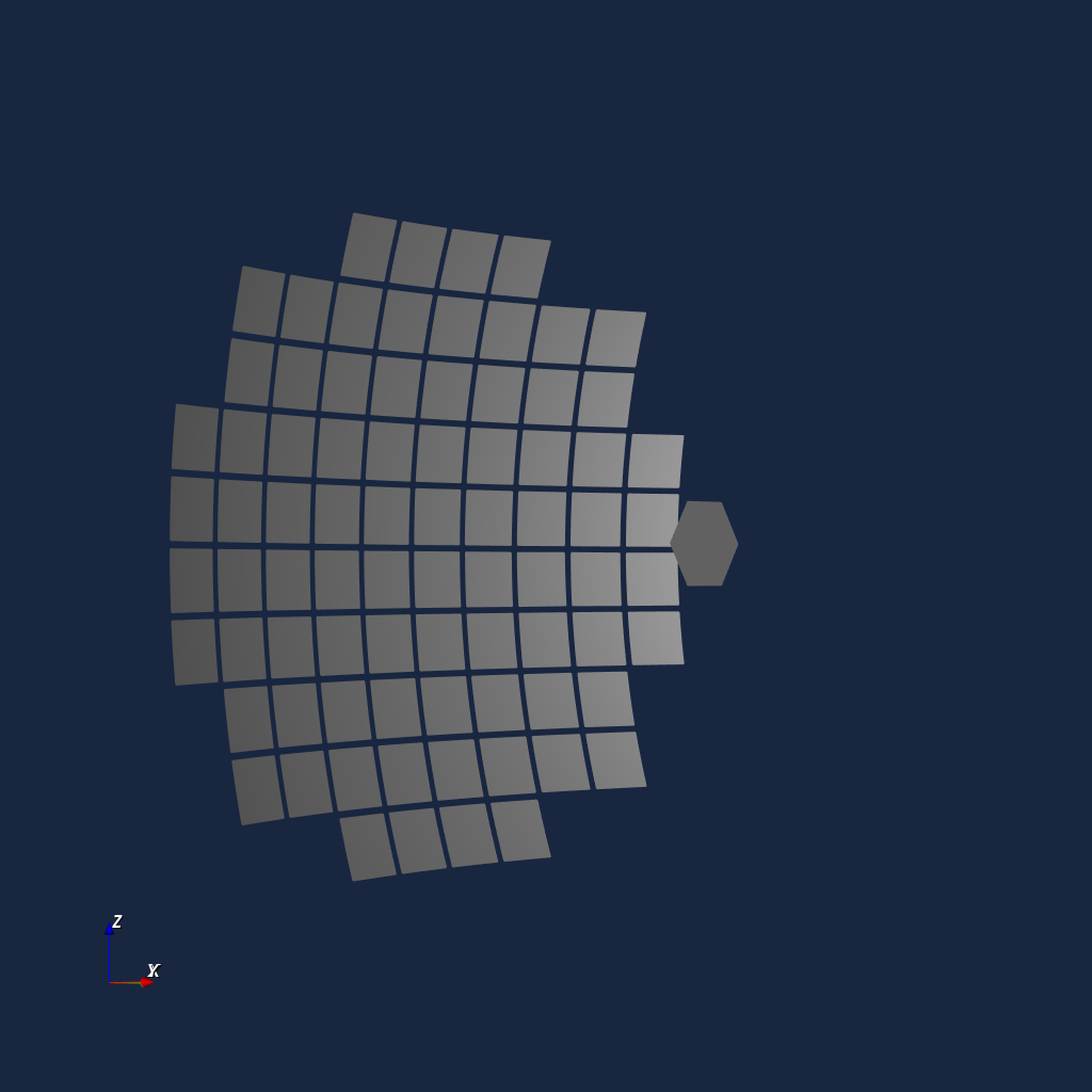
Visualize your geometry
For optical systems with complex geometry, it is often useful to perform a visual check of the geometry. To do so, a VTK visualizer is provided:
renderer = iactsim.visualization.VTKOpticalSystem(segmented_telescope.optical_system)
renderer.start_render()
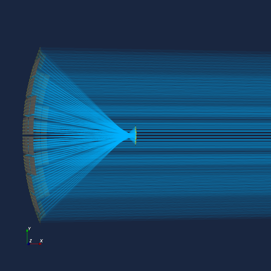
Visualize ray-tracing
segmented_telescope.visualize_ray_tracing(*source.generate(10000))
For developers
Release history Release notifications | RSS feed


Download files
Download the file for your platform. If you're not sure which to choose, learn more about installing packages.
Source Distribution
File details
Details for the file iactsim-0.12.0.tar.gz.
File metadata
- Download URL: iactsim-0.12.0.tar.gz
- Upload date:
- Size: 2.8 MB
- Tags: Source
- Uploaded using Trusted Publishing? No
- Uploaded via: twine/6.2.0 CPython/3.12.3
File hashes
| Algorithm | Hash digest | |
|---|---|---|
| SHA256 |
b0f7703f8ee332f41ba69a3065ff5d5edfc347e838b5853aa913e58beb25928f
|
|
| MD5 |
dad0e5a4e8ed69e21033a8c01c2edb2e
|
|
| BLAKE2b-256 |
e3a7846bb398d66e82482669aa47888ccb78568b30c99cfe2c6289f9c523435e
|


