Imaging Atmospheric Cherenkov Telescopes simulation

Project description
iactsim: Imaging Atmospheric Cherenkov Telescope Simulation
GPU-accelerated instrument response simulation for IACTs.
Documentation | Source Code | Report Bug
Overview
iactsim is a high-performance Python package designed for simulating the response of Imaging Atmospheric Cherenkov Telescopes (IACTs). By exploiting the parallel computational power of GPUs (via CUDA and CuPy), it accelerates computationally intensive tasks such as ray-tracing and SiPM response simulation.
Package Structure
The framework is organized into four main modules:
- optics: handles optical system and camera geometry definitions, non-sequential ray-tracing, and photon sources.
- electronics: manages pixel signal generation trigger logic, and sampling logic. Currently only SiPMs are supported, including prompt cross-talk, after-pulse and micro-cell recovery time
- visualization: provides tools for 3D geometry/ray-tracing rendering (via VTK) and helper matplotlib functions for data plotting.
- iactxx: a general-purpose C++ extension module for high-performance parallel reading, decompression, and conversion of files written with the IACT extension of CORSIKA7.
Key Features
- GPU Acceleration: accelerated performance for ray-tracing and camera response simulation using NVIDIA HPC SDK and CuPy.
- Flexible Optics:
- non-sequential ray-tracing algorithm supporting multiple reflections (e.g., protective windows, multi-layer coatings);
- currently supports spherical, aspherical, flat and cylindrical surfaces;
- complex geometries including mirror segmentation with customizable alignment errors (tilts/shifts).
- Advanced Electronics:
- detailed SiPM response simulation (prompt cross-talk, after-pulse and microcell recovery time);
- run-time configuration of pixel properties on a per-pixel basis;
- flexible trigger and sampling logic customization.
- Visualization:
- built-in plotting capabilities for the detailed analysis of ray-tracing results and camera electronic signals;
- 3D interactive visualization of optical systems and photon paths using VTK.
- Python-based: seamless integration with the scientific Python stack (NumPy, SciPy, Numba, Matplotlib, Jupyter, etc.).
Table of Contents
Installation
Prerequisites
- Python: >= 3.11
- Compiler: gcc (standard) or nvcc (optional)
- CMake: >= 3.15
- Runtime: NVIDIA Drivers, CUDA, CuPy
1. Environment setup
We strongly recommend using a virtual environment (e.g., mamba or conda):
mamba create -n simenv python=3.13
mamba activate simenv
2. Install via PyPI
If you have the prerequisites installed, you can install the latest release directly:
pip install iactsim -v
Optional: using NVHPC compilers
Building with gcc is the standard and requires no special configuration. However, if you specifically wish to use the nvcc, you must configure the environment before installation.
Please refer to the NVIDIA HPC SDK section in Runtime Configuration for detailed instructions on setting up the environment.
Custom Compiler Flags
You can customize the build options by passing arguments to CMake via pip. The following flags are available:
- CMAKE_CXX_COMPILER=<compiler>: specify the C++ compiler executable (e.g., nvcc, g++).
- USE_ZLIBNG=<ON|OFF>: enable/disable zlib-ng support. Default is ON.
For the C++ part, by default zlib-ng (zlib data compression library for the next generation systems) will be used (CMake will clone the repo automatically). This is strongly recommended if you plan to read compressed CORSIKA files.
If you have to use the standard system zlib, you can set this to OFF.
Example: explicitly use nvcc and disable zlib-ng
python -m pip install . -v -C cmake.args="-DCMAKE_CXX_COMPILER=nvcc;-DUSE_ZLIBNG=OFF"
Install from source
-
Clone the repository:
git clone https://gitlab.com/davide.mollica/iactsim.git
cd iactsim
-
Editable install:
First, install the build dependencies required for the editable install:pip install scikit-build-core pybind11 "setuptools_scm[toml]>=8.0" cmake ninja
Then, install the package in editable mode. This configuration disables build isolation, ensuring that only modified C++ files will be recompiled:
python -m pip install --no-build-isolation -e .
Runtime Configuration
1. Install CuPy (required)
iactsim relies on CuPy for GPU offloading. You must install the cupy package that matches your specific CUDA version.
pip install cupy-cuda<XXX>
Replace <XXX> with your CUDA version (e.g., cupy-cuda12x for CUDA 12).
For detailed instructions, refer to the CuPy documentation.
2. NVIDIA HPC SDK (optional)
If you are using the NVIDIA HPC SDK to provide CUDA libraries, you must configure the enviroment so that CuPy can locate the necessary libraries (you can download HPC SDK from the NVIDIA website).
We suggest to use Environment Modules to handle SDK configuration and then define NVCC and CUDA_PATH enviromental variables:
module load nvhpc
export NVCC=$NVHPC_ROOT/compilers/bin/nvcc
export CUDA_PATH=$NVHPC_ROOT/cuda
With conda/mamba enviroments you can use the provided configuration script configure_conda_env
mamba activate simenv
configure_conda_env simenv
mamba deactivate
This adds an activation script and a deactivation script to the simenv enviroment that will automatically handle the configuration when it is activated or deactivated.
Usage
Building an optical system
The following code provides an example of how to build a simple optical system with a spherical mirror and a flat focal surface.
import matplotlib.pyplot as plt
import iactsim
from iactsim.optics import (
ApertureShape,
SurfaceType,
OpticalSystem,
)
# Use iactsim matplotlib style
plt.style.use('iactsim.iactsim')
# Spherical mirror
mirror_curvature_radius = 20000
plate_scale = mirror_curvature_radius/57.296/2.
mirror = iactsim.optics.SphericalSurface(
half_aperture=10000.,
curvature=1./mirror_curvature_radius,
position=(0,0,0),
# reflective in the pointing direction
surface_type=SurfaceType.REFLECTIVE_FRONT,
name = 'Mirror'
)
# Flat focal surface (5deg hexagon)
focal_plane = iactsim.optics.FlatSurface(
half_aperture = 5*plate_scale,
position = (0,0,0.5*mirror_curvature_radius),
aperture_shape = ApertureShape.HEXAGONAL,
# sensitive surface opposite to the pointing direction
surface_type=SurfaceType.SENSITIVE_BACK,
name = 'Focal Plane'
)
# Optical system
os = OpticalSystem(
surfaces=[focal_plane, mirror],
name='TEST-OS'
)
# Telescope position
pos = (0,0,0)
# Telescope pointing (alt,az)
poi = (0.,0.)
# IACT
telescope = iactsim.IACT(
os,
position=pos,
pointing=poi
)
# Copy optical system data to the device
telescope.cuda_init()
# Photon source initialized on-axis
source = iactsim.optics.sources.Source(telescope)
source.positions.random = False # To make spot diagrams
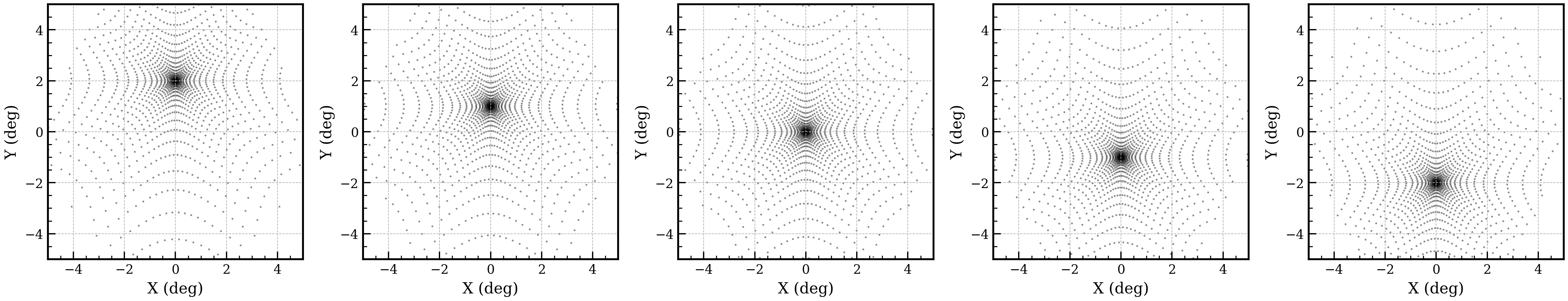
# Plot spot diagram at different off-axis angles
n_plots = 5
fig, axes = plt.subplots(1,n_plots,figsize=(3.5*n_plots,3.5))
source.directions.altitude = telescope.altitude - 2.
for ax in axes:
# Adjust photon position to match the mirror position
source.set_target('Mirror')
# Generate photons
ps, vs, wls, ts = source.generate(10000)
# Perform ray-tracing
telescope.trace_photons(ps, vs, wls, ts)
# Plot spot diagram
iactsim.visualization.scatter(ps, s=0.2, ax=ax, color='black', alpha=0.5, scale=plate_scale)
ax.set_xlabel('X (deg)')
ax.set_ylabel('Y (deg)')
ax.grid(ls='--')
# Move the source
source.directions.altitude += 1. # degree
plt.tight_layout()
plt.show()
Mirror segmentation
The following code provides an example of how to segment a surface (AsphericalSurface, SphericalSurface or FlatSurface)
starting from a mother surface (in this case mirror).
Note that each segment is an independent surface and does not need a mother surface, which is used here simply for convenience.
import numpy as np
# List of segments
segments = []
# Segment ID
k = 0
# Segments on a 10X10 grid, 80 total
n = 10
segment_distance = 2*mirror.half_aperture / (n+3)
for i in range(n+3):
for j in range(n+3):
offset = [
-mirror.half_aperture+segment_distance*i,
-mirror.half_aperture+segment_distance*j
]
r_segment = np.sqrt(offset[0]**2+offset[1]**2)
# Do not create segments outside the original mirror aperture
if r_segment > mirror.half_aperture-segment_distance*np.sqrt(2):
continue
# Ideal segment position
segment_position = [
offset[0],
offset[1],
mirror.sagitta(r_segment),
]
# Create the surface
segment = iactsim.optics.SphericalSurface(
curvature=mirror.curvature,
half_aperture=0.45*segment_distance,
position=segment_position,
surface_type=mirror.type,
name = f'Segment-{k}',
aperture_shape=ApertureShape.SQUARE,
# Big random dispersion for visualization purpose
tilt_angles=np.random.normal(0,1,3),
# Gaussian scattering
scattering_dispersion=0.05
)
# Specify the segment offset
# When a segment is created in this way:
# - it will be oriented with the same surface normal
# of the mother surface at the specified offset
# - `tilt_angles` attribute will define a deviation from this orientation.
segment.offset = offset
segments.append(segment)
k += 1
# Optical system
segmented_os = iactsim.optics.OpticalSystem(
surfaces=[focal_plane, *segments],
name='SEGMENTED-TEST-OS'
)
# IACT
segmented_telescope = iactsim.IACT(segmented_os, position=pos, pointing=poi)
segmented_telescope.cuda_init()
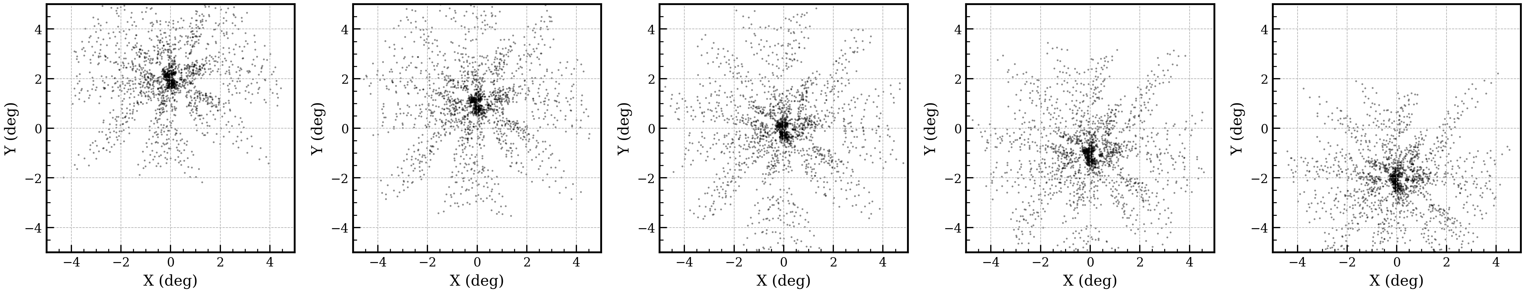
# Plot spot diagram at different off-axis angles
n_plots = 5
fig, axes = plt.subplots(1,n_plots,figsize=(3.5*n_plots,3.5))
# Photon source initialized on-axis
source = iactsim.optics.sources.Source(segmented_telescope)
source.positions.radial_uniformity = False
source.positions.random = False
source.positions.r_max = mirror.half_aperture*1.5
source.directions.altitude -= 2.
for ax in axes:
# Adjust photon position to match the mirror position
source.set_target()
# Generate photons
ps, vs, wls, ts = source.generate(10000)
# Perform ray-tracing
segmented_telescope.trace_photons(ps, vs, wls, ts)
# Plot spot diagram
iactsim.visualization.scatter(ps, s=0.2, ax=ax, color='black', alpha=0.5, scale=plate_scale)
ax.set_xlabel('X (deg)')
ax.set_ylabel('Y (deg)')
ax.grid(ls='--')
# Move the source
source.directions.altitude += 1. # degree
plt.tight_layout()
plt.show()
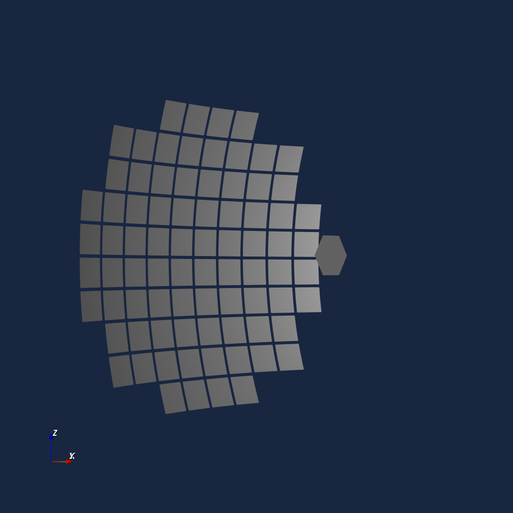
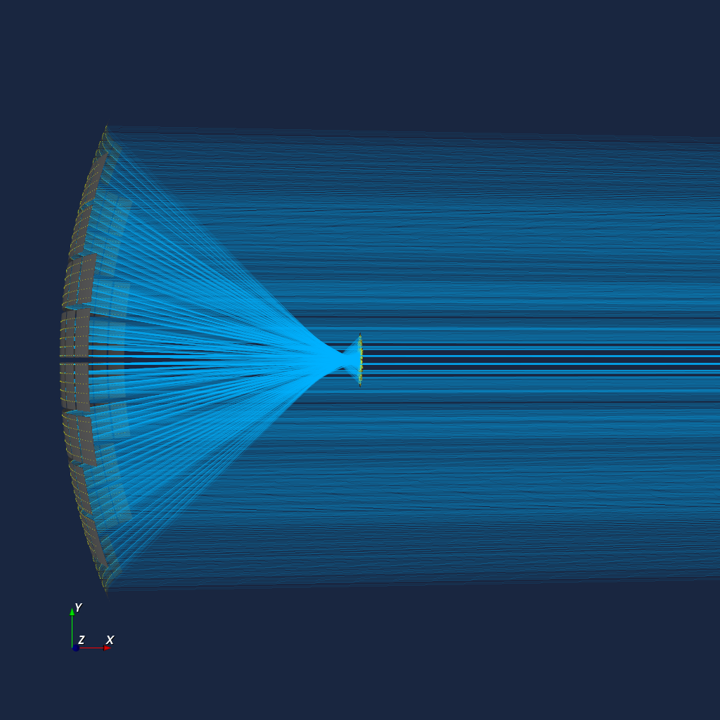
3D Visualization
Verify your geometry or visualize ray-tracing paths using the built-in VTK backend.
Interactive 3D view of the optical system
from iactsim.visualization import VTKOpticalSystem
renderer = VTKOpticalSystem(segmented_telescope.optical_system)
renderer.start_render()
Visualize ray paths
segmented_telescope.visualize_ray_tracing(
    *source.generate(10000),
    map_wavelength_color=False,
    focal_point='FocalPlane',
    show_not_detected=False
)
For Developers
- Performance Benchmarks: Current vs Main Branch
- Contributions: Contributions are welcome! Please open an issue before submitting a MR.
Release history Release notifications | RSS feed


Download files
Download the file for your platform. If you're not sure which to choose, learn more about installing packages.
Source Distribution
File details
Details for the file iactsim-0.13.1.tar.gz.
File metadata
- Download URL: iactsim-0.13.1.tar.gz
- Upload date:
- Size: 2.3 MB
- Tags: Source
- Uploaded using Trusted Publishing? No
- Uploaded via: twine/6.2.0 CPython/3.12.3
File hashes
| Algorithm | Hash digest | |
|---|---|---|
| SHA256 |
f3280bea3b4d4830e817285d80d7515fefd349d51ca43722f552e0ec976fe29b
|
|
| MD5 |
5f0a0c14298f50c0dcae1806a3384856
|
|
| BLAKE2b-256 |
8999fa675fb5fc3094d8af2d8f420caffdcdb083493327df68e58cfe453b3743
|


